Spreadsheet Equations Explained: How to Turn Real-World Problems into Formulas in Excel

Last updated: July 27, 2026

Quick Answer: Spreadsheet equations in Excel are instructions that tell a cell how to calculate a value using data from other cells. To turn a real-world problem into a formula, break the problem into its parts (what you know, what you need), map each part to a cell, then connect them with Excel functions and operators. Most real problems, budgets, commissions, attendance, can be solved with fewer than five core functions.

Key Takeaways

Every Excel formula starts with = and references cells instead of fixed numbers wherever possible.
Absolute references ($A$1) lock a cell address when copying; relative references (A1) shift automatically.
IF, SUMIF, VLOOKUP, and IFERROR solve the majority of real-world calculation problems.
Translate word problems into formulas by identifying inputs, outputs, and the rule connecting them.
Common beginner mistakes include hardcoding numbers, mixing up absolute/relative references, and skipping error handling.
Array formulas calculate across ranges in one step but need careful syntax (Ctrl+Shift+Enter in older Excel versions).
Cross-sheet formulas use SheetName!CellAddress syntax to pull data from other tabs.
Naming cells and adding comments makes complex formulas far easier to audit and reuse.

What Is a Spreadsheet Formula and How Does It Work?

A spreadsheet formula is a calculation instruction stored in a cell. When Excel sees the = sign at the start of a cell entry, it evaluates everything after it as a math expression, a function call, or a combination of both, then displays the result.

Every formula has three possible ingredients:

Operators, +, -, *, /, ^ (exponent), & (join text)
Cell references, A1, B3:B20, Sheet2!C5
Functions, built-in commands like SUM(), IF(), VLOOKUP()

How it processes: Excel reads the formula left to right, respects standard order of operations (parentheses first, then exponents, then multiply/divide, then add/subtract), and recalculates automatically whenever a referenced cell changes.

💡 Quick example: A cell containing =B2+B3 adds whatever is in B2 and B3. Change B2 from 100 to 150, and the result updates instantly, no manual recalculation needed.

For a deeper foundation, see this beginner-to-advanced guide on how to write spreadsheet formulas.

How Do I Write a Formula to Solve a Real Problem in Excel?

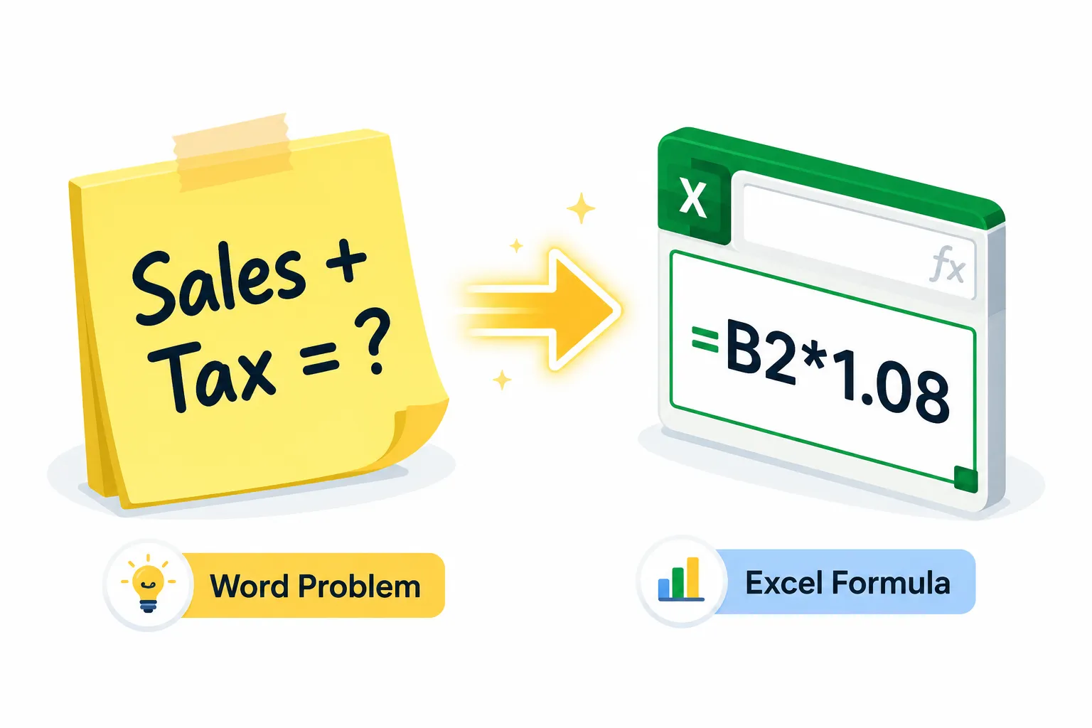
The key is to translate the word problem into a logical sentence before touching the keyboard. Think: “What do I know? What do I need? What’s the rule connecting them?”

A three-step thinking pattern works for almost every scenario:

Identify inputs, What raw numbers or text exist already? Put each in its own cell.
State the rule in plain English, “Commission equals sales multiplied by the rate.”
Map the rule to formula syntax, =C2*D2 (where C2 = sales, D2 = rate).

Worked example, Sales commission tracker:

Column	Label	Value
A	Rep Name	Jordan
B	Sales	8500
C	Rate	0.07
D	Commission	`=B2*C2` → $595

Worked example, Project timeline days remaining:

A project manager needs to know how many days are left before a deadline. The formula is simply: =D2-TODAY() where D2 holds the deadline date. Excel stores dates as numbers, so subtraction works natively.

For more step-by-step worked examples across real workflows, check out Master Spreadsheet Equations in Excel.

What’s the Difference Between Absolute and Relative Cell References?

Relative references (A1) shift when a formula is copied to another cell. Absolute references ($A$1) stay fixed no matter where the formula moves. Mixing them up is the single most common source of wrong results when copying formulas down a column.

=B2*C2, both references shift when copied down (relative)
=B2*$C$1, B2 shifts, but $C$1 always points to the tax rate in row 1 (mixed)
=SUM($B$2:$B$20), the range never changes (absolute)

Choose absolute references when the formula needs to always point to a fixed lookup value, a tax rate, or a company-wide constant stored in one cell.

Choose relative references when the formula should repeat the same logic row by row (like calculating each employee’s pay from their own row of data).

Press F4 while clicking a cell reference in the formula bar to cycle through all four reference modes.

How Do I Calculate Percentages in Excel?

Percentages in Excel are just decimal multiplication. Excel stores 15% as 0.15, so =B2*15% and =B2*0.15 produce the same result.

Common percentage formulas:

Percent of total: =B2/SUM($B$2:$B$10), note the absolute reference on the SUM range
Percent change: =(New-Old)/Old → format the cell as a percentage
Adding tax: =Price*(1+TaxRate) e.g., =B2*(1+0.08)
Discount: =Price*(1-DiscountRate) e.g., =B2*(1-0.2)

⚠️ Common mistake: Dividing by a relative reference when calculating percent of total. If the denominator shifts when you copy the formula down, every row gets a different total. Lock it with $.

What Formulas Should I Use for Budgeting and Expense Tracking?

For budgeting and expense tracking, five formulas cover nearly every scenario: SUM, SUMIF, IF, IFERROR, and basic arithmetic for variance.

Core budget formula set:

Formula	Use case	Example
`SUM`	Total all expenses in a category	`=SUM(B2:B30)`
`SUMIF`	Total only expenses matching a label	`=SUMIF(A2:A30,"Food",B2:B30)`
`IF`	Flag over-budget rows	`=IF(D2>E2,"Over","OK")`
`IFERROR`	Prevent ugly error messages	`=IFERROR(C2/D2,0)`
Variance	Actual vs. budget difference	`=Actual-Budget`

For a ready-to-use financial model, see How to Find and Use a Profit and Loss Statement Template in Excel 365.

When Should I Use SUMIF Instead of Regular SUM?

Use SUMIF (or SUMIFS for multiple conditions) whenever the total should only include rows that meet a specific criterion. Regular SUM adds everything in a range regardless of content.

SUMIF syntax: =SUMIF(range, criteria, sum_range)

range, the column Excel checks (e.g., category labels)
criteria, what to match (e.g., “Marketing”, “>500”, a cell reference)
sum_range, the column to add up when the condition is met

Example, Attendance tracking:

To count total hours worked only by part-time staff: =SUMIF(C2:C50,"Part-Time",D2:D50)

SUMIFS extends this to multiple conditions: =SUMIFS(D2:D50,C2:C50,"Part-Time",E2:E50,"January")

Can I Use IF Statements to Create Conditional Calculations?

Yes, IF is one of the most powerful tools for turning real-world decision logic into spreadsheet equations. It evaluates a condition and returns one value if true, another if false.

Syntax: =IF(logical_test, value_if_true, value_if_false)

Worked example, Sales commission tiers:

A rep earns 5% on sales under $5,000 and 8% on sales of $5,000 or more:

=IF(B2>=5000, B2*0.08, B2*0.05)

Nested IF for three tiers:

=IF(B2>=10000, B2*0.10, IF(B2>=5000, B2*0.08, B2*0.05))

Keep nesting to a maximum of two or three levels for readability. For more complex logic, IFS (available in Excel 2019+) is cleaner: =IFS(B2>=10000, B2*0.10, B2>=5000, B2*0.08, TRUE, B2*0.05)

How Do I Use VLOOKUP to Pull Data from Another Table?

VLOOKUP searches the first column of a table for a match and returns a value from a specified column in the same row. It’s the go-to formula for pulling product prices, employee data, or tax brackets from a reference table.

Syntax: =VLOOKUP(lookup_value, table_array, col_index_num, [range_lookup])

lookup_value, what to search for (e.g., a product ID)
table_array, the reference table range (lock it with $)
col_index_num, which column in the table to return (1 = first column)
range_lookup, use FALSE for exact match (almost always what you want)

Example: Pull a product price from a price list on Sheet2:

=VLOOKUP(A2, Sheet2!$A$2:$C$100, 2, FALSE)

💡 Tip: Excel 365 users can use XLOOKUP instead, it’s more flexible, handles errors gracefully, and doesn’t require the lookup column to be first.

For more on building reusable lookup structures, see Spreadsheet Equations for Real Analytics.

How Do I Use VLOOKUP to Pull Data from Another Table?

How Do I Troubleshoot a Formula That Shows an Error?

Excel error codes are diagnostic messages, not failures. Each one points to a specific problem.

Error	Meaning	Quick fix
`#DIV/0!`	Dividing by zero or empty cell	Wrap in `IFERROR` or check the denominator
`#VALUE!`	Wrong data type (text where number expected)	Check source cells for hidden spaces or text
`#REF!`	A referenced cell was deleted	Re-enter the formula with valid references
`#NAME?`	Excel doesn’t recognize a function name	Check spelling; confirm function exists in your version
`#N/A`	VLOOKUP can’t find a match	Use `IFERROR` or verify the lookup value exists
`#NUM!`	Invalid numeric operation	Check for negative square roots or out-of-range values

Debugging workflow:

Click the cell with the error.
Use Formulas → Evaluate Formula to step through the calculation.
Press Ctrl + [ to jump to all cells the formula references.
Wrap the whole formula in IFERROR(formula, "Check data") as a temporary diagnostic.

What’s the Best Way to Organize Complex Formulas for Readability?

Break complex formulas into helper columns and use named ranges. A formula that spans 200 characters is hard to audit and nearly impossible to hand off to a colleague.

Practical strategies:

Helper columns: Calculate intermediate results in separate columns, then reference those columns in the final formula. Label each helper column clearly.
Named ranges: Select a cell or range, type a name in the Name Box (top-left), and use that name in formulas. =Revenue-COGS reads better than =B2-C2.
Line breaks in formulas: In the formula bar, press Alt+Enter to add visual line breaks inside long formulas, Excel ignores them but they help during editing.
Comments: Right-click any cell → Insert Comment to document what a formula does and why.

For advanced techniques on building formulas that scale, see Spreadsheet Formulas for Advanced Users.

What Common Mistakes Do Beginners Make When Writing Formulas?

The most damaging beginner mistake is hardcoding numbers inside formulas instead of referencing cells. When the tax rate changes from 8% to 9%, a hardcoded formula requires a manual hunt through every cell. A cell-referenced formula updates everywhere at once.

Top five beginner mistakes:

Hardcoding values, Use =B2*$D$1 not =B2*0.08
Forgetting to lock references, Causes formulas to drift when copied
Circular references, A formula that references its own cell causes an infinite loop
Mixing data types, Numbers stored as text won’t sum correctly; use Data → Text to Columns to convert
No error handling, Bare formulas break visibly; wrap risky divisions in IFERROR

How Do I Automate Calculations for Inventory or Sales Tracking?

For inventory and sales tracking, the combination of SUMIF, IF, and structured Excel Tables (Ctrl+T) creates a near-automatic calculation system. Excel Tables auto-expand formulas to new rows, so adding a sale or stock entry updates all totals instantly.

Basic inventory formula set:

Stock remaining: =Opening_Stock + Received - Sold
Reorder alert: =IF(D2<E2,"Reorder","OK") (D2 = current stock, E2 = reorder point)
Total sales value: =SUMPRODUCT(Units_Sold, Unit_Price)

For repetitive multi-step processes, Excel Macros can record and replay actions automatically. See how to enable macros in Excel to get started.

What’s the Difference Between Array Formulas and Regular Formulas?

A regular formula calculates one result from one set of inputs. An array formula calculates across an entire range in a single step, often replacing what would otherwise require dozens of helper columns.

Example: Count sales over $500 in a range without a helper column:

Regular approach: Add a helper column with =IF(B2>500,1,0) then SUM it.
Array formula: =SUM(IF(B2:B50>500,1,0)), entered with Ctrl+Shift+Enter in Excel 2016 and earlier (Excel 365 handles most arrays automatically with dynamic array functions).

Dynamic array functions (Excel 365 only) like FILTER, SORT, and UNIQUE spill results into neighboring cells automatically, making many old array formula tricks unnecessary.

⚠️ Edge case: In older Excel versions, forgetting Ctrl+Shift+Enter on an array formula returns only the first value in the range, not the full calculation.

How Do I Create a Formula That Works Across Multiple Sheets?

Cross-sheet formulas use the syntax SheetName!CellAddress. To reference cell B5 on a sheet named “January,” write =January!B5. To sum the same cell across multiple sheets (a 3D reference), use =SUM(January:March!B5).

Practical cross-sheet scenario, Monthly budget rollup:

Each month lives on its own sheet (January, February, March). A summary sheet pulls totals:

=SUM(January:December!B2), adds cell B2 from every sheet between January and December.

Tips for cross-sheet formulas:

Sheet names with spaces need single quotes: ='Q1 Sales'!B5
Use INDIRECT to build sheet names dynamically from cell values (advanced)
Keep sheet structures identical across tabs so 3D references stay accurate

FAQ

Q: What’s the fastest way to sum a column in Excel? Select the cell below the column, press Alt + =, and Excel inserts a SUM formula automatically. See the Excel AutoSum shortcut guide for more detail.

Q: Can I use text as a condition in SUMIF? Yes. Use the criteria argument with text in quotes: =SUMIF(A2:A30,"Marketing",B2:B30). Wildcards work too: "Mar*" matches “Marketing,” “March,” and “Margin.”

Q: How do I stop a formula from recalculating automatically? Go to Formulas → Calculation Options → Manual. Press F9 to recalculate on demand. Use this only for very large workbooks that slow down on every keystroke.

Q: What’s the difference between VLOOKUP and INDEX/MATCH? VLOOKUP requires the lookup column to be the leftmost column in the table. INDEX(MATCH()) can look up in any direction and is generally more flexible. In Excel 365, XLOOKUP replaces both.

Q: How do I reference a cell on another sheet in a formula? Type =, click the other sheet tab, click the cell, and press Enter. Excel writes the cross-sheet reference automatically in the format =SheetName!CellAddress.

Q: Why does my formula show the formula text instead of a result? The cell is formatted as Text. Select the cell, change the format to General (Home → Number Format), then re-enter the formula by pressing F2 and Enter.

Q: How do I copy a formula without changing the cell references? Either use absolute references ($A$1) before copying, or copy the cell, paste it using Paste Special → Formulas, which preserves the formula text exactly.

Q: What’s the easiest way to find all formulas in a spreadsheet? Press Ctrl + ` (grave accent) to toggle formula view, showing all formulas instead of results. Press it again to return to normal view.

Q: Can Excel formulas handle dates and times? Yes. Excel stores dates as serial numbers (days since January 1, 1900), so date arithmetic works naturally. =TODAY() returns today’s date; =NOW() includes the current time.

Q: When should I use a Pivot Table instead of formulas? Use a Pivot Table when you need to summarize, group, or filter a large dataset interactively without writing formulas. Formulas are better for fixed calculations that feed into other formulas. See Excel Pivot Tables for 2026 for a full walkthrough.

Conclusion

Translating real-world problems into spreadsheet equations is a skill built on a simple habit: slow down, state the problem in plain English, then map each word to a cell or function. The formulas themselves aren’t the hard part, the thinking pattern is.

Actionable next steps:

Pick one real task you currently do by hand (a budget, a commission sheet, an attendance log) and rebuild it in Excel using cell references instead of hardcoded numbers.
Master five core functions first: SUM, IF, SUMIF, VLOOKUP, and IFERROR. These cover roughly 80% of everyday business calculations.
Add error handling to every formula that divides or looks up data, wrap it in IFERROR from day one.
Use named ranges for any value referenced in more than three formulas. Your future self will thank you.
Explore further with the step-by-step examples for real workflows and the beginner-friendly Excel guide to keep building from here.

The goal isn’t to memorize every function, it’s to develop the instinct for breaking any problem into inputs, a rule, and an output. Once that thinking pattern clicks, every new formula becomes straightforward.