How to Fix Excel Formulas That Return Errors: The Most Common Causes and Solutions

Last updated: July 30, 2026

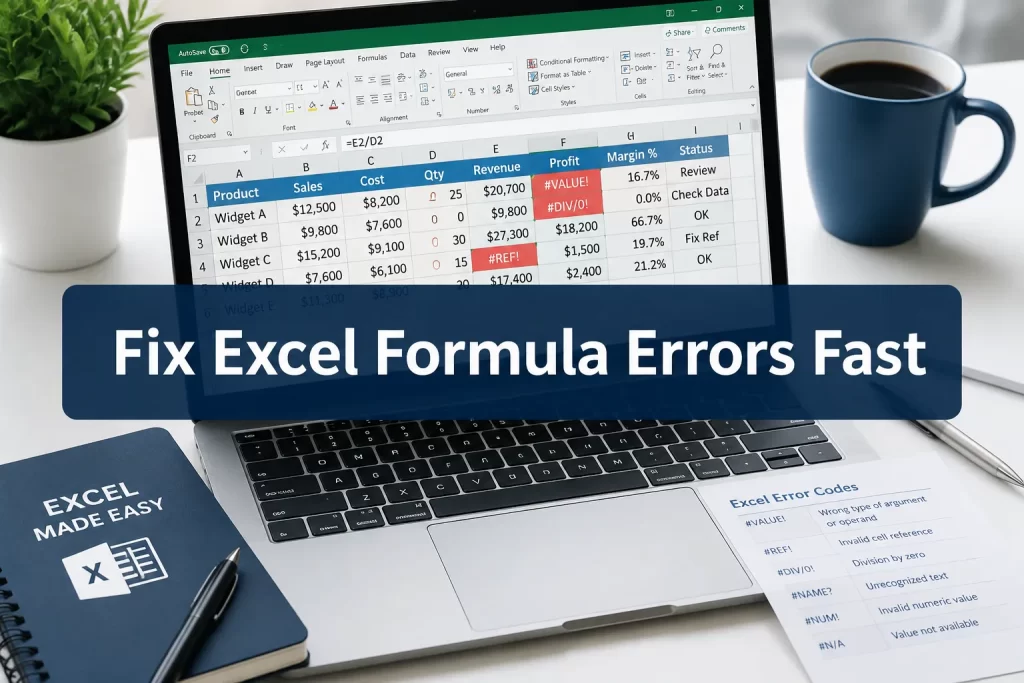
Quick Answer: Excel formula errors like #VALUE!, #REF!, #DIV/0!, #N/A, and #NAME? each have a specific cause. Knowing what each error code means is the fastest way to fix it. Use Excel’s built-in Error Checking tool (Formulas tab → Error Checking) to locate and step through each issue, then apply the targeted fix for that error type.

Key Takeaways

Excel recognizes 11 distinct error values in 2026, including newer ones like #SPILL! and #CALC! introduced with dynamic arrays [2]
#VALUE! means wrong data type; #REF! means a cell reference no longer exists; #DIV/0! means division by zero
#NAME? usually means a typo in a function name or a missing named range
#N/A means a lookup found no match, not always a true error
Use Formulas → Error Checking or press F9 to step through and debug complex formulas [1]
The IFERROR function lets you replace any error with a custom message or blank cell
Circular references stop Excel from calculating correctly, find them under Formulas → Error Checking → Circular References
Formulas returning wrong results (no error shown) are often caused by calculation mode set to Manual or mismatched cell formats
Background error checking (File → Options → Formulas) flags issues with green triangles before they cause bigger problems [1]
Consistent formula patterns, structured tables, and named ranges prevent most errors before they start [8]

What Does #VALUE! Error Mean in Excel?

#VALUE! appears when a formula receives the wrong data type, for example, trying to add a number to a text cell. It’s one of the most common errors in Excel and usually points to a mismatch between what the formula expects and what’s actually in the referenced cells.

Common causes:

A cell contains text (including a space) where a number is expected
Date cells formatted as text rather than actual date values
Extra spaces in cells that look empty but aren’t
Array formulas applied to incompatible ranges

How to fix it:

Click the cell with the error and check the formula bar
Trace each referenced cell, look for text formatted as numbers or hidden spaces
Use =TRIM() to remove extra spaces, or =VALUE() to convert text-numbers to real numbers
If the error comes from a specific argument, select that part of the formula in the formula bar and press F9 to see what it evaluates to [4]

Quick example: =A1+B1 returns #VALUE! if B1 contains the word “N/A” instead of a number. Fix: clean B1’s data or wrap the formula: =IFERROR(A1+B1, 0).

How to Fix #REF! Error in Excel Formulas

#REF! means a formula is pointing to a cell that no longer exists. This happens most often after deleting rows, columns, or sheets that were referenced in a formula.

Common causes:

Deleting a row or column that a formula depended on
Cutting and pasting cells in a way that breaks references
Copying a formula that uses relative references outside its valid range

Fix steps:

Click the error cell and look at the formula bar, you’ll see #REF! where the broken reference sits
Press Ctrl+Z to undo the deletion if it just happened
Otherwise, manually correct the reference to point to the right cell or range
Use Formulas → Trace Precedents to visually map what the formula was referencing [1]

Edge case: If a formula references another sheet that was renamed or deleted, you’ll also get #REF!. Re-link the formula to the correct sheet name.

For more on building solid formulas from the start, see this beginner-to-advanced guide to writing spreadsheet formulas.

Why Is My Excel Formula Returning #DIV/0! Error?

#DIV/0! appears whenever a formula tries to divide a number by zero or by an empty cell. Excel can’t compute division by zero, so it flags it immediately.

Fix options:

Check whether the denominator cell is empty or contains a zero
Use IFERROR to handle it gracefully: =IFERROR(A1/B1, "No data")
Use an IF check: =IF(B1=0, 0, A1/B1)

This error is especially common in financial models and percentage calculations where source data hasn’t been filled in yet.

What Causes #NAME? Error in Excel

#NAME? means Excel doesn’t recognize something in the formula, usually a function name with a typo, or a named range that doesn’t exist.

Most common causes:

Misspelled function name (e.g., =VLOKUP instead of =VLOOKUP)
Using a function from an add-in that isn’t enabled (like Analysis ToolPak) [10]
Referencing a named range that was deleted or never created
Forgetting to put text strings in quotation marks
Regional separator issues, some Windows configurations use semicolons instead of commas in formulas [10]

Fix: Start typing the function name and let Excel’s autocomplete confirm the correct spelling. Check Formulas → Name Manager to verify named ranges exist.

How to Troubleshoot #N/A Error in Spreadsheets

#N/A means “not available”, a lookup formula (VLOOKUP, HLOOKUP, MATCH, XLOOKUP) couldn’t find the value it was searching for. This isn’t always a mistake; sometimes it correctly signals missing data.

Causes and fixes:

Cause	Fix
Lookup value doesn’t exist in the table	Verify the source data or use approximate match
Extra spaces in lookup value or table	Use `=TRIM()` on both sides
Data types don’t match (text vs. number)	Convert with `=VALUE()` or reformat the column
Exact match required but not set	Set match type to `0` (exact) in MATCH/VLOOKUP

Wrap with IFERROR if you want blanks instead of errors: =IFERROR(VLOOKUP(A1, B:C, 2, 0), "").

What’s the Difference Between #NULL! and #VALUE! Errors

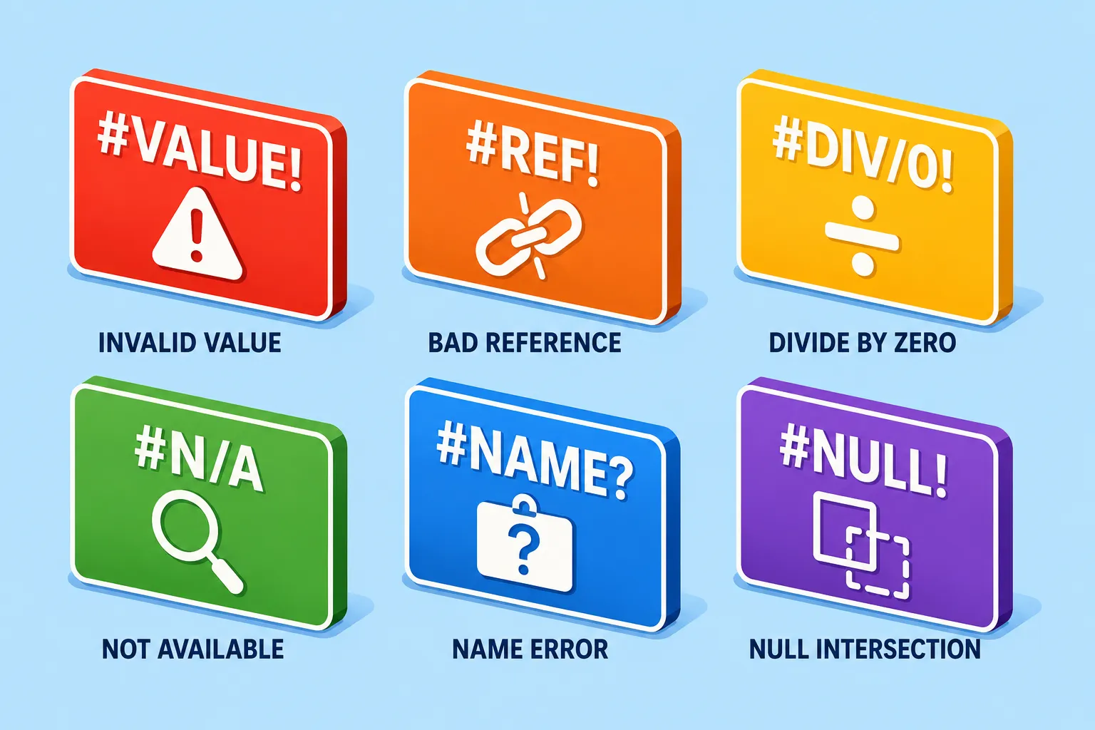
#NULL! and #VALUE! are both formula errors, but they have different causes. #NULL! is specifically caused by using a space (the intersection operator) between two ranges that don’t actually intersect, for example, =SUM(A1:A5 C1:C5). #VALUE! is broader and covers any type mismatch or invalid argument.

In practice: #NULL! is rare and almost always caused by a missing comma or colon in a range reference. If you see it, check for accidental spaces between range references in the formula.

Excel Formula Error Checking Tools and How to Use Them

Excel has several built-in tools that make finding and fixing errors much faster. Using them is the professional approach to debugging, especially in large workbooks. [1]

Key tools:

Error Checking dialog (Formulas → Error Checking): Steps through each error in the sheet one by one, with options to fix, ignore, or get help [1]
Evaluate Formula (Formulas → Formula Auditing → Evaluate Formula): Walks through each step of a formula’s calculation so you can see exactly where it breaks [4]
Trace Precedents / Trace Dependents: Draws arrows showing which cells feed into a formula and which cells depend on it [8]
Show Formulas (Ctrl + `): Displays all formulas instead of results, making it easy to spot inconsistencies across a range [1]
Background error checking: Enable via File → Options → Formulas → “Enable background error checking”, flags issues with a green triangle as you work [1]

Pro tip: Press F9 while a sub-expression is selected in the formula bar to preview its value without committing the change. Always press Esc afterward to avoid overwriting the formula with a static value [4].

For a broader look at Excel productivity, check out Excel keyboard shortcuts for busy professionals, many of the auditing tools have fast keyboard access.

How to Debug Complex Excel Formulas Step by Step

Debugging a long nested formula is much easier when broken into stages. The goal is to isolate which part of the formula is failing.

Step-by-step debug checklist:

✅ Click the error cell and read the formula bar in full
✅ Open Evaluate Formula (Formulas tab) and click “Evaluate” repeatedly to step through each calculation
✅ Select individual sub-expressions in the formula bar and press F9 to check their output [4]
✅ Break the formula into smaller helper cells temporarily to test each piece
✅ Check that all referenced ranges exist and are the right size
✅ Verify data types match what the function expects
✅ Press Esc when done to restore the original formula

This approach works for any error type and is especially useful for nested IF, INDEX/MATCH, or array formulas.

If you’re applying formulas across large datasets, see how to insert a formula in Excel for an entire column for best practices that reduce reference errors.

How to Fix Circular Reference Errors in Excel

A circular reference happens when a formula refers back to its own cell, either directly or through a chain of other cells. Excel can’t resolve this loop and either shows a warning or returns 0. [14]

How to find them:

Go to Formulas → Error Checking → Circular References, Excel lists every cell involved
The status bar at the bottom of the screen also shows “Circular References” when one exists

How to fix them:

Rethink the formula logic so the cell doesn’t reference itself
If intentional (iterative calculation), enable it under File → Options → Formulas → “Enable iterative calculation”, but use this carefully

Common mistake: Accidentally including the result cell in a SUM range. For example, putting =SUM(A1:A10) in cell A10 creates a circular reference. Fix by changing the range to =SUM(A1:A9).

Can I Hide Error Values in Excel Instead of Fixing Them?

Yes, sometimes an error is expected (like #N/A in a lookup that hasn’t been filled in yet) and hiding it is perfectly reasonable. The best tool for this is IFERROR.

Using IFERROR:

<code>=IFERROR(your_formula, value_if_error)
</code>

Examples:

=IFERROR(VLOOKUP(A1,B:C,2,0),"Not found"), shows text instead of #N/A
=IFERROR(A1/B1, 0), shows 0 instead of #DIV/0!
=IFERROR(formula, ""), shows a blank cell

When to hide vs. fix: Hide errors when they’re expected and harmless (incomplete data entry, optional lookups). Fix errors when they indicate real data problems that could affect totals, reports, or decisions.

You can also use conditional formatting to visually flag error cells without hiding them, useful for quality-checking large datasets. See how to use conditional formatting traffic lights in Excel for a practical approach.

Excel Formula Returning Wrong Result But No Error Message

This is often trickier than a visible error because Excel doesn’t flag it. The formula runs, but the answer is wrong.

Most common causes:

Calculation mode set to Manual: Formulas don’t recalculate automatically. Fix: File → Options → Formulas → set to “Automatic”, or press F9 to force recalculation [14]
Cell formatted as Text: Excel treats the formula as a text string and displays it literally. Fix: reformat the cell as General or Number, then re-enter the formula
Mismatched absolute/relative references: A formula copied across rows or columns picks up the wrong cells. Use $ to lock references where needed
Hidden rows or columns included in a range: SUM or AVERAGE may include data you can’t see
Numbers stored as text: Cells look like numbers but are left-aligned, they won’t calculate. Use Data → Text to Columns or =VALUE() to convert them

Quick check: Press Ctrl + ` (grave accent) to toggle Show Formulas mode and scan for any formula that looks different from its neighbors in the same column.

For related data-quality issues, how to find duplicates in Excel covers another common source of unexpected results in large datasets.

Best Practices to Prevent Formula Errors in Excel

The best way to handle formula errors is to prevent them in the first place. These habits reduce errors significantly in day-to-day spreadsheet work. [8]

Prevention checklist:

📋 Use Excel Tables (Ctrl+T): Structured references auto-adjust when rows are added or deleted, eliminating most #REF! errors
📋 Use named ranges: =SUM(SalesData) is harder to break than =SUM(B2:B100)
📋 Validate input data: Use Data Validation to restrict cells to numbers, dates, or list values, this prevents #VALUE! errors at the source
📋 Keep formulas consistent across rows: Use Show Formulas to spot inconsistencies before they cause problems [1]
📋 Wrap risky formulas in IFERROR: Especially for lookups and division
📋 Enable background error checking: Green triangles catch issues early [1]
📋 Avoid merging cells in data ranges: Merged cells break many formulas, see how to merge cells in Excel for when it’s safe to use this feature

For a deeper dive into building reliable calculation models, spreadsheet equations for real analytics covers reusable formula architecture in both Excel and Google Sheets.

Best Practices to Prevent Formula Errors in Excel

FAQ: How to Fix Excel Formulas That Return Errors

Q: Why does my formula show the formula text instead of a result? The cell is formatted as Text. Select it, change the format to General (Home → Number Format), then press F2 and Enter to re-evaluate.

Q: What’s the fastest way to find all errors in a worksheet? Press Ctrl+G → Special → Formulas → check “Errors only” → OK. Excel selects every error cell at once.

Q: Can IFERROR hide all error types? Yes. IFERROR catches every Excel error type, #VALUE!, #REF!, #N/A, #DIV/0!, #NAME?, #NULL!, #NUM!, and the newer #SPILL! and #CALC! errors.

Q: What is a #SPILL! error? #SPILL! appears when a dynamic array formula tries to return results into a range that’s blocked by existing data. Clear the cells in the spill range to fix it [2].

Q: How do I stop Excel from recalculating constantly? If recalculation is slowing you down, set it to Manual (File → Options → Formulas → Manual) and press F9 when you’re ready to update. Just remember to switch back to Automatic before sharing the file [14].

Q: Why does VLOOKUP return #N/A even when the value exists? Usually a data type mismatch (one cell is text, the other is a number) or trailing spaces. Use =TRIM() and =VALUE() to clean both the lookup value and the table column.

Q: What does #NUM! mean? #NUM! means a formula contains an invalid numeric value, for example, trying to find the square root of a negative number, or a date calculation that produces a number outside Excel’s valid date range.

Q: How do I fix a formula that worked yesterday but errors today? Check whether source data was deleted or moved (#REF!), whether the calculation mode changed to Manual, or whether an add-in was disabled [10]. Also check if a referenced sheet was renamed.

Q: Is there a way to audit all formulas in a workbook at once? Yes. Use Formulas → Formula Auditing → Error Checking to step through every error. For a full audit, the Inquire add-in (available in Excel for Microsoft 365) provides a workbook analysis report.

Q: Can circular references ever be intentional? Yes, iterative calculations (like compound interest models) sometimes need circular references. Enable them under File → Options → Formulas → “Enable iterative calculation” and set a maximum iteration count.

Conclusion: Your Practical Debug Checklist for Excel Formula Errors

Understanding how to fix Excel formulas that return errors comes down to reading the error code, using the right tool, and fixing the root cause rather than just masking it. Here’s the action plan:

Identify the error type, each code (#VALUE!, #REF!, #DIV/0!, #N/A, #NAME?, #SPILL!) points directly at the problem
Use Error Checking (Formulas tab) to step through every issue in the sheet [1]
Evaluate complex formulas one step at a time using the Evaluate Formula tool or F9 [4]
Wrap expected errors in IFERROR to keep reports clean
Fix the data source when errors point to missing, misformatted, or deleted data
Enable background error checking so green triangles catch new issues early [1]
Build with Tables and named ranges to prevent most reference errors from happening at all [8]

For anyone just getting started with Excel, the how to use Excel with formulas guide is a solid foundation before tackling error troubleshooting.

References

[1] Detect Formula Errors In Excel – https://support.microsoft.com/en-us/excel/detect-formula-errors-in-excel [2] Article – https://www.microsoftpressstore.com/articles/article.aspx?p=3131362 [4] Article – https://www.microsoftpressstore.com/articles/article.aspx?p=2955139&seqNum=2 [8] How To Find Errors In Excel Formulas – https://www.journalofaccountancy.com/issues/2024/jun/how-to-find-errors-in-excel-formulas/ [10] techcommunity.microsoft – https://techcommunity.microsoft.com/discussions/excelgeneral/why-do-i-keep-getting-a-pesky-formula-error-message/4074326