GROUPBY and PIVOTBY in Excel: Build Dynamic Reports Without PivotTables (2026 Hands-On Guide)

Last updated: July 31, 2026

Quick Answer: GROUPBY and PIVOTBY are two powerful Excel functions introduced in Microsoft 365 that let you summarize and cross-tabulate data using a single formula, without building a PivotTable. They update automatically when your data changes, support dynamic arrays, and give you formula-level control over how results are sorted, filtered, and formatted. This guide walks through both functions with hands-on examples for 2026.

Key Takeaways 🎯

• GROUPBY summarizes data by one or more row categories (like SUMIF, but far more flexible).
• PIVOTBY adds a column dimension, producing a two-way cross-tab, think PivotTable in a formula.
• Both functions require Microsoft 365 (current channel); they are not available in Excel 2021 or earlier standalone versions.
• Results spill automatically into adjacent cells using Excel’s dynamic array engine.
• Unlike PivotTables, these formulas refresh instantly, no right-click “Refresh” needed.
• You can nest other functions (LAMBDA, FILTER, SORT) inside them for advanced reporting.
• Common mistakes include forgetting to lock array references and mixing data types in group columns.
• For beginners still learning the basics, check out how to use Excel with formulas before diving in.

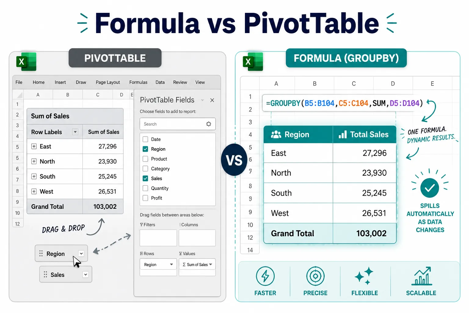
What Is the GROUPBY Function in Excel and How Does It Work?

GROUPBY groups rows of data by one or more category columns and applies an aggregation function (like SUM, COUNT, or AVERAGE) to return a summarized result. It works like a smarter SUMIF that can handle multiple grouping levels and multiple value columns at once.

Syntax

<code>=GROUPBY(row_fields, values, function, [field_headers], [total_depth], [sort_order], [filter_array])
</code>

Argument	What It Does
row_fields	The column(s) to group by (e.g., a Region column)
values	The column(s) to aggregate (e.g., Sales amounts)
function	The aggregation: SUM, COUNT, AVERAGE, MAX, etc.
field_headers	0 = no headers, 1 = headers without totals, 2 = headers with totals
total_depth	Controls subtotals and grand totals
sort_order	Positive = ascending, negative = descending
filter_array	Optional TRUE/FALSE array to pre-filter rows

Quick Example

Say column A has product categories and column B has sales figures:

<code>=GROUPBY(A2:A100, B2:B100, SUM)
</code>

This returns a two-column spill: one column of unique categories, one column of their summed sales. No PivotTable wizard needed.

“GROUPBY is essentially a formula-driven PivotTable row section, fast, live, and fully nestable.”

GROUPBY Excel Syntax and Examples: Multiple Columns and Real Scenarios

GROUPBY supports multiple grouping columns by passing an array of columns as the first argument. This makes it easy to group by, say, both Region and Product in one formula.

Group by Two Columns

<code>=GROUPBY(A2:B100, C2:C100, SUM, 1, 1)
</code>

Here, column A is Region, column B is Product, and column C is Revenue. The result spills a three-column summary with a grand total row.

Use GROUPBY Instead of SUMIF

If you’ve been writing chains of SUMIF formulas to build summary tables, GROUPBY replaces all of them in one cell. For example, instead of:

<code>=SUMIF($A$2:$A$100, "North", $C$2:$C$100)
=SUMIF($A$2:$A$100, "South", $C$2:$C$100)
</code>

…you write one GROUPBY formula and let it spill the full summary automatically. This is covered in more detail in the section on when to use GROUPBY instead of SUMIF below.

Common mistake: Selecting only part of your data range. Always include all rows, or better yet, format your data as an Excel Table (Ctrl+T) so the range expands automatically.

How to Use the PIVOTBY Function in Excel with Dynamic Arrays

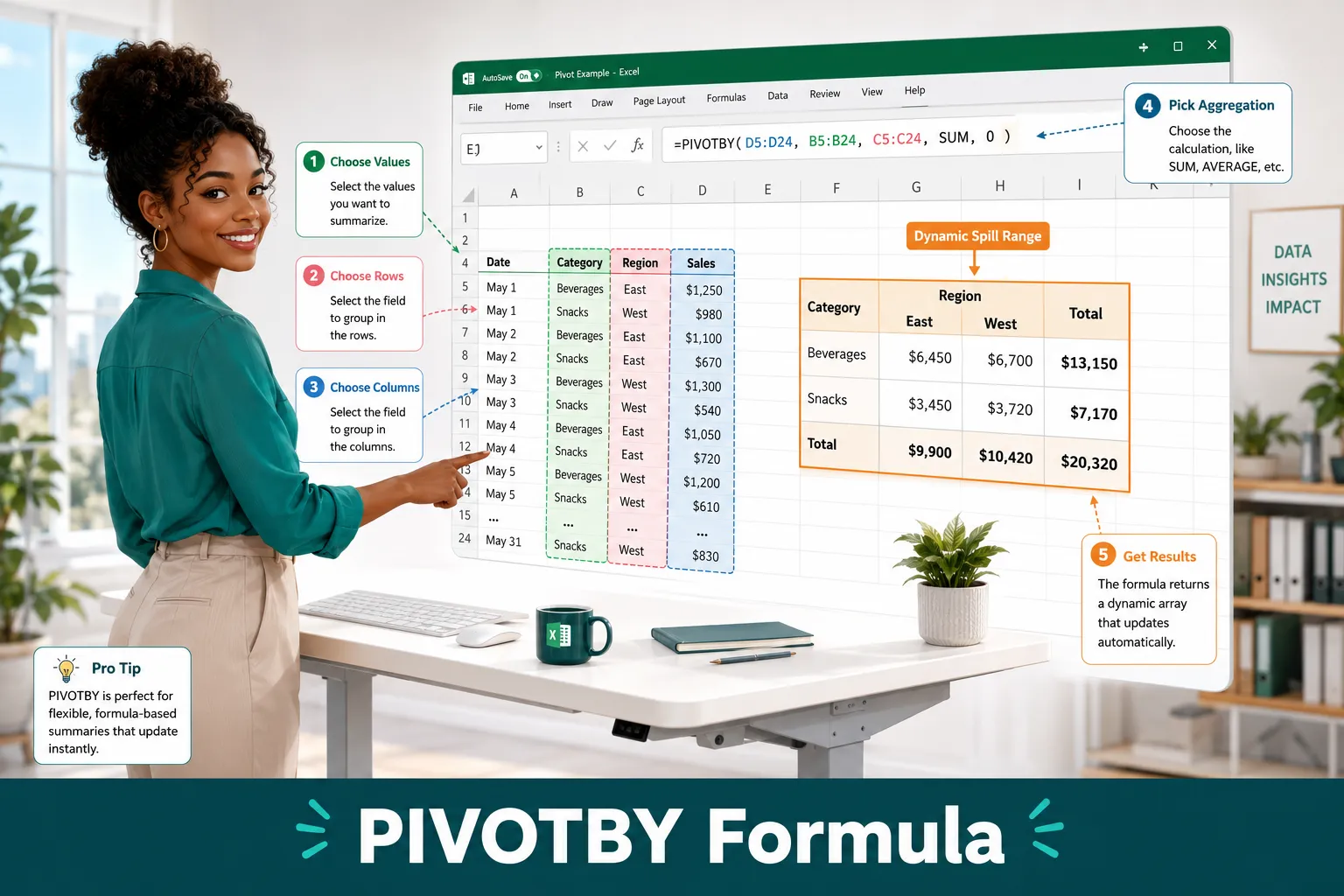
PIVOTBY extends GROUPBY by adding a column-grouping argument, creating a two-dimensional cross-tab, rows grouped one way, columns grouped another. It’s the formula equivalent of a PivotTable’s row and column fields combined.

Syntax

<code>=PIVOTBY(row_fields, col_fields, values, function, [field_headers], [row_total_depth], [col_total_depth], [sort_order], [filter_array])
</code>

Example: Sales by Region and Quarter

<code>=PIVOTBY(A2:A100, B2:B100, C2:C100, SUM, 1, 1, 1)
</code>

• Column A: Region (row grouping)
• Column B: Quarter (column grouping)
• Column C: Sales (values)

The result spills a grid: regions down the rows, quarters across the columns, totals on the edges. It updates the moment you add a new row of data.

When to Use PIVOTBY vs. GROUPBY

• Use GROUPBY when you need a one-dimensional summary (rows only).
• Use PIVOTBY when you need a two-dimensional cross-tab (rows AND columns).

If you’re already comfortable with Excel Pivot Tables, think of GROUPBY as the “Row Labels” area and PIVOTBY as “Row Labels + Column Labels” combined into one formula.

Difference Between GROUPBY and PivotTable in Excel

The core difference is control and automation: GROUPBY and PIVOTBY live inside formulas, so they recalculate instantly and can be combined with other functions. PivotTables are interactive UI objects that require a manual refresh when source data changes.

Here’s a practical comparison:

Feature	PivotTable	GROUPBY / PIVOTBY
Refreshes automatically	❌ Manual refresh	✅ Yes
Nestable in other formulas	❌ No	✅ Yes
Drag-and-drop interface	✅ Yes	❌ Formula only
Conditional formatting	✅ Easy	✅ Possible
Works in older Excel	✅ Yes	❌ Microsoft 365 only
Custom sort/filter in formula	❌ Limited	✅ Built-in arguments

Choose a PivotTable if your audience needs to interact with slicers and drill-downs without touching formulas. Choose GROUPBY/PIVOTBY if you want a live, formula-driven report that feeds into dashboards or other calculations.

Can GROUPBY Replace Pivot Tables in Excel?

GROUPBY and PIVOTBY can replace PivotTables for most reporting tasks, but not all. For read-only summary reports that update automatically, they’re often a better choice. For interactive exploration with slicers, drill-through, and visual grouping, PivotTables still have the edge.

Scenarios where GROUPBY/PIVOTBY win:

• Reports embedded inside larger formula-driven dashboards
• Summaries that feed into charts automatically (see how to turn Excel data into a chart quickly)
• Situations where you need the output to be a live spill range, not a static object
• Reports shared with users who shouldn’t accidentally break a PivotTable layout

Scenarios where PivotTables still win:

• Business users need point-and-click filtering with slicers
• You need drill-down to underlying rows
• Your team isn’t comfortable with formulas

Excel GROUPBY Function Not Available: What Version Do You Need?

GROUPBY and PIVOTBY require Microsoft 365 (current channel) on Windows or Mac. They are not available in Excel 2019, Excel 2021, or any perpetual-license version of Excel.

• ✅ Microsoft 365 Personal, Family, Business, or Enterprise (current channel)
• ✅ Excel for the web (Office.com), partial support as of 2026
• ❌ Excel 2021 (standalone)
• ❌ Excel 2019 or earlier
• ❌ Google Sheets (no equivalent native function)

To check your version: Go to File → Account → About Excel. If your build number is 2302 or later and you’re on the current channel, you should have both functions.

If GROUPBY still doesn’t appear, type =GROUPBY( in a cell. If Excel doesn’t autocomplete it, your channel may be on Semi-Annual (SAC) rather than Current Channel. Ask your IT admin to switch channels, or use Excel for the web as a workaround.

How to Create Dynamic Reports with GROUPBY and PIVOTBY

Building a dynamic report with GROUPBY and PIVOTBY in Excel is straightforward when you follow a clear structure. Here’s a step-by-step approach that works for sales, budget, or any tabular dataset.

Step 1: Format your data as a Table Select your data and press Ctrl+T. Name the table (e.g., SalesData). This ensures your GROUPBY formula always includes new rows.

Step 2: Write your GROUPBY formula In an empty area of your sheet:

<code>=GROUPBY(SalesData[Region], SalesData[Revenue], SUM, 1, 1, -2)
</code>

The -2 in sort_order sorts by value descending, highest revenue region first.

Step 3: Add a PIVOTBY for the cross-tab view

<code>=PIVOTBY(SalesData[Region], SalesData[Quarter], SalesData[Revenue], SUM, 1, 1, 1)
</code>

Step 4: Connect to a chart Click any cell in the spill range, then press Alt+F1 to instantly create a chart. Because the spill range updates automatically, your chart updates too.

For more on building budget-style reports, the monthly food budget template guide shows how structured tables power live summaries.

GROUPBY Not Working in Excel: Troubleshooting Common Issues

Most GROUPBY errors come from mismatched range sizes, mixed data types in the grouping column, or spill range conflicts. Here are the most common problems and fixes:

• #VALUE! error: The values range and row_fields range have different row counts. Make sure both start and end on the same rows.
• #SPILL! error: Something is blocking the spill range (a value in an adjacent cell). Clear the cells below and to the right of your formula.
• #NAME? error: The function isn’t available in your Excel version. See the version requirements above.
• Blank rows in output: Your grouping column has empty cells. Filter them out using the filter_array argument: =GROUPBY(A2:A100, B2:B100, SUM,,A2:A100<>"").
• Totals not showing: Set field_headers to 2 and total_depth to 1.
• Wrong sort order: Use positive integers for ascending, negative for descending in the sort_order argument.

GROUPBY Excel When to Use Instead of SUMIF

Use GROUPBY instead of SUMIF when you have multiple categories to summarize, need sorted output, or want the result to update as new categories appear. SUMIF requires you to know every category in advance and write one formula per category. GROUPBY discovers all unique categories automatically.

Situation	Best Choice
One known category, one sum	SUMIF
All categories, auto-discovered	GROUPBY
Two-dimensional summary	PIVOTBY
Need result inside another formula	GROUPBY
Excel 2019 or earlier	SUMIF (only option)

For users still building foundational formula skills, the step-by-step Excel formula guide is a good starting point before tackling GROUPBY.

GROUPBY and PIVOTBY Excel 2026: New Features and What’s Changed

In 2026, Microsoft has continued refining GROUPBY and PIVOTBY with better support for LAMBDA helper functions, improved performance on large datasets, and expanded aggregation options. As of mid-2026, notable additions include:

• PERCENTOF as a built-in aggregation option inside GROUPBY, showing each group’s share of the total without a separate formula.
• Improved spill range stability when used inside named ranges or structured table references.
• Better integration with FILTER and SORT, nesting these inside GROUPBY’s filter_array argument is now more predictable.
• Excel for the web has caught up significantly, supporting most GROUPBY/PIVOTBY arguments that previously only worked in the desktop app.

These improvements make the case for GROUPBY and PIVOTBY in Excel: Build Dynamic Reports Without PivotTables even stronger heading into late 2026.

FAQ: GROUPBY and PIVOTBY in Excel

Q: Does GROUPBY work with text values (COUNT) or only numbers (SUM)? Yes. Use COUNTA for text or mixed columns, COUNT for numbers only, and SUM for numeric totals. All standard aggregation functions work.

Q: Can I use GROUPBY inside an IF formula? Yes. Because GROUPBY returns a spill array, you can wrap it in other array-aware functions. However, using it directly inside a traditional IF may cause errors, use IFS or IFERROR as a wrapper instead.

Q: How do I add a grand total row to GROUPBY output? Set the total_depth argument to 1 for a grand total, or 2 for subtotals at each group level.

Q: Can PIVOTBY show percentages instead of raw numbers? Yes. Use PERCENTOF as the function argument (available in current Microsoft 365 builds as of 2026), or divide the PIVOTBY result by a total using a second formula.

Q: Will GROUPBY slow down Excel on large datasets? On datasets under ~500,000 rows, performance is generally fast. For very large datasets, consider using Power Query to pre-aggregate before using GROUPBY on the summarized output.

Q: Can I use GROUPBY on a filtered table? Yes, use the filter_array argument to pass a TRUE/FALSE array that mirrors your filter logic. This is more reliable than relying on Excel’s AutoFilter state.

Q: Is there a way to sort GROUPBY results by value, not by category name? Yes. Use -2 in the sort_order argument to sort by value descending, or 2 for ascending. Use 1 or -1 to sort alphabetically by the group label.

Q: Does PIVOTBY support multiple value columns? Yes. Pass an array of columns as the values argument: SalesData[Revenue]:SalesData[Units] to get both metrics in the cross-tab.

Q: Can I connect a GROUPBY result to a chart? Yes. Select any cell in the spill range and insert a chart normally. The chart will update automatically when the underlying data changes, no refresh needed.

Q: What happens if I add a new category to my data? If your source is formatted as an Excel Table, GROUPBY automatically picks up the new category in its output the moment you add the row. No formula editing required.

Conclusion: Start Building Smarter Reports Today

GROUPBY and PIVOTBY in Excel: Build Dynamic Reports Without PivotTables represent a genuine shift in how Excel handles data summarization. For anyone who has spent time wrestling with PivotTable refresh buttons, layout resets, or chains of SUMIF formulas, these two functions are a practical upgrade worth learning in 2026.

Actionable next steps:

1. Check your Excel version, confirm you’re on Microsoft 365 current channel.
2. Format your data as a Table (Ctrl+T) before writing any GROUPBY formula.
3. Start with GROUPBY on a simple one-column grouping to get comfortable with the syntax.
4. Move to PIVOTBY once you’re confident, try a Region × Quarter sales cross-tab.
5. Connect your spill range to a chart for a fully live, auto-updating dashboard.
6. Explore nesting, combine GROUPBY with FILTER or SORT for more targeted reports.

For a deeper dive into traditional PivotTable techniques that still have their place, the Excel Pivot Tables step-by-step guide is worth bookmarking alongside this one. And if you’re newer to Excel overall, how to use Excel for beginners step by step builds the foundation that makes GROUPBY and PIVOTBY click faster.