
Click here to view our video tutorial
Click here to download our PDF tutorial
Drop-down lists are one of the simplest ways to make a spreadsheet faster to fill out and harder to mess up. Instead of typing a status, category, or label into a cell by hand every time, you click a small arrow and pick from a preset list of choices. No typos, no inconsistent spelling, no “In Progress” in one row and “in progress” in another. It’s a small change that makes a big difference once you’re relying on that data for sorting, filtering, or reporting.
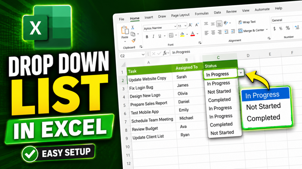
Excel builds this feature right in through a tool called Data Validation, and you don’t need any formulas or add-ins to use it. You simply tell Excel which cells should have a drop-down, and then tell it what options should appear in that list. The list can be anything you want: task statuses, department names, yes or no answers, product categories, whatever fits your spreadsheet.
In this guide, we’ll walk through exactly how to turn an empty column into a working drop-down list, using a simple task tracker as our example. By the end, every cell in that column will have its own set of ready-to-pick options.
Getting to Know Your Starting Data
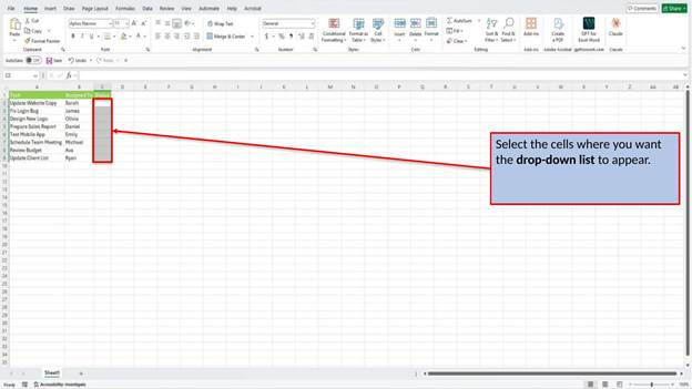
Before we get into the steps, take a look at the list we’re starting with. It has a Task column, an Assigned To column, and a Status column, and right now that Status column is completely empty. That’s exactly the situation Data Validation is built for: turning a blank column into a fast, consistent, click-to-choose field.
Step 1: Select the Cells For Your Drop-Down List
Click and drag to select the cells where you want the drop-down list to appear. This can be a single cell or an entire range, depending on what you need. In our example, we’re selecting every cell in the Status column so that each task gets its own drop-down.
Step 2: Open the Data Tab and Click Data Validation
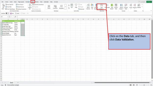
With your cells still selected, click on the Data tab in the ribbon at the top of Excel. In the Data Tools group, you’ll find a button labeled Data Validation. Click it, and a dialog box opens where you’ll set up the rules for your list.
Step 3: Set Allow to List and Enter Your Options
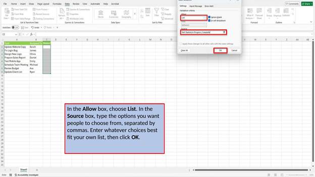
In the dialog box, click the Allow dropdown and choose List. A new box labeled Source will appear. This is where you type the options you want people to choose from, separated by commas. You can enter whatever choices best fit your own list; ours uses Not Started, In Progress, and Complete, but yours might be department names, yes or no, or anything else. Once you’ve typed your options, click OK.
Step 4: Look For the Drop-Down Arrow
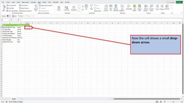
As soon as you click OK, a small arrow appears on the right side of each selected cell. That arrow is your sign that the drop-down list is active and ready to use.
Step 5: Click the Arrow and Choose an Option
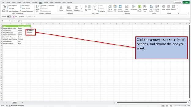
Click the arrow on any cell, and the full list of options you entered will drop down right below it. Click the one you want, and it fills in the cell instantly, no typing required.
Step 6: Fill In the Rest of Your List
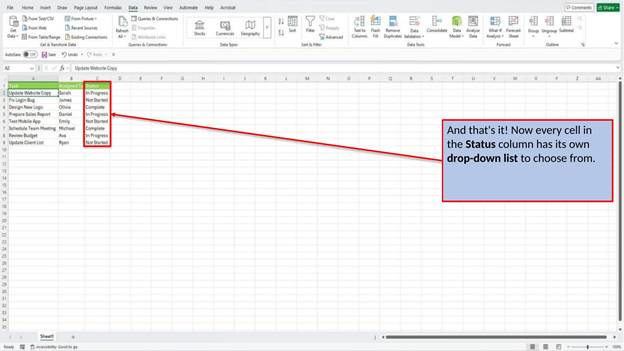
Repeat that same click-and-choose process for the rest of the cells, and you’ll end up with a column that’s fully consistent from top to bottom. Every entry comes from the same set of options, so there’s no risk of stray typos or mismatched wording sneaking into your data.
And that’s all it takes to add a drop-down list to your spreadsheet. Data Validation isn’t limited to status columns either; it works just as well for anything with a fixed set of options, from yes-or-no fields to department names to product categories. The next time you catch yourself typing the same handful of values over and over, set up a drop-down list instead and let Excel do the consistency checking for you.
Video Tutorial
Download PDF Below