
Click here to view our video tutorial
Click here to download our PDF tutorial
If you’ve ever imported data from a CSV file, copied numbers from a website, or typed a leading apostrophe into a cell, there’s a good chance some of your “numbers” in Excel aren’t really numbers at all. They’re text that just happens to look like numbers. The telltale signs are easy to miss at first: totals that add up to zero, numbers that line up on the left side of the cell instead of the right, and formulas that seem to ignore certain cells entirely.
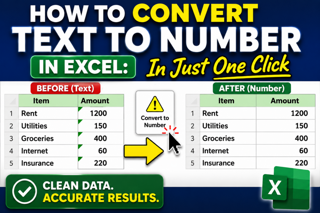
The good news is that Excel already knows when this happens, and it gives you a fast way to fix it. Whenever you select a cell containing a number stored as text, a small warning icon pops up right next to it. That icon isn’t just a warning, it’s also a shortcut. Click it, and Excel will convert the text back into a real, calculable number in a single click.
In this guide, we’ll walk through exactly how to spot the warning icon and use it to convert text to numbers, using a simple list of monthly expenses as our example. Along the way, we’ll also cover what to do if that icon doesn’t show up for you, or if you’re working with far more data than you’d want to fix one click at a time.
Getting to Know Your Starting Data
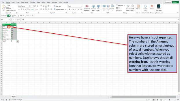
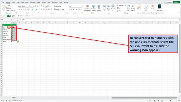
Before we get into the steps, take a look at the list we’re starting with. It has an Item column and an Amount column listing common monthly expenses like Rent, Utilities, and Groceries. At a glance, everything looks normal, but the Amount column is actually storing every value as text instead of as a number. One easy way to spot the problem: the Total row currently shows 0, because Excel can’t add up numbers that aren’t really numbers.
Step 1: Watch For Excel’s Warning Icon
Click on any cell that contains a number stored as text, and Excel displays a small yellow warning icon just to the side of it. This icon is part of Excel’s built-in error checking, and it’s specifically designed to flag numbers that are formatted as text. It’s easy to overlook if you’re not looking for it, but once you know it’s there, it’s the key to fixing the whole column in seconds.
Step 2: If You Don’t See The Warning Icon
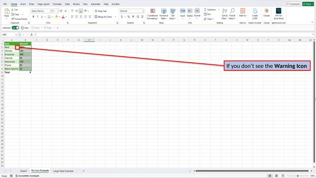
The warning icon only appears if Excel’s error checking for text-formatted numbers is turned on, and it only shows up when you actually have a cell with this issue selected. If you select your own text-stored numbers and don’t see the icon, that setting may be turned off, or you may be looking at a different kind of formatting issue altogether. Either way, there’s another reliable method that doesn’t depend on that icon at all: the Paste Special method.
Step 3: Or You Have A Large Amount Of Data To Convert
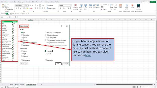
Clicking a warning icon works great for a handful of cells, but it isn’t practical if you’re converting hundreds or thousands of rows at once. For that situation, the Paste Special method lets you convert an entire large range to numbers in just a few clicks, no matter how much data you’re working with. We cover that method step by step in our companion tutorial.
Step 4: Select The Cells You Want To Fix
Click and drag to select the cells containing the numbers you want to convert. This can be a single cell or an entire column, depending on what you’re working with. As soon as you make your selection, the warning icon appears, letting you know Excel has recognized the text-stored numbers and is ready to fix them.
Step 5: Click The Warning Icon, Then Convert To Number
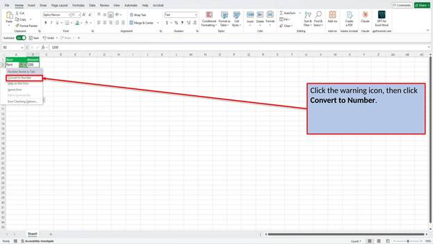
Click the warning icon, and a small menu opens with a handful of options. Choose Convert to Number, and Excel instantly changes every cell in your selection from text into an actual, calculable number. No formulas, no retyping, and no separate dialog boxes to click through.
Step 6: Check Your Converted Numbers
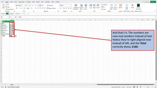
Take a look at your data now. The numbers shift to the right side of their cells, which is Excel’s default alignment for actual numbers (text stays left-aligned, which is one more way to spot the issue in the future). And the Total row, which showed 0 before, now correctly adds up to 2160.
And that’s all it takes to convert text to numbers in Excel. This trick isn’t limited to expense lists either, it works just as well on data imported from a CSV file, pasted from a website, or entered with a leading apostrophe, anywhere Excel is quietly storing your numbers as text. The next time your totals don’t add up the way they should, look for that small warning icon and let Excel do the fixing for you.
Video Tutorial
Download PDF Below