
Click here to view our video tutorial
Click here to download our PDF tutorial
If you’ve ever imported a large amount of data from a CSV file, an accounting system, or a website, there’s a good chance some of those “numbers” in Excel aren’t actually numbers at all. They’re text that just happens to look like numbers.

The telltale signs are easy to spot once you know what to look for: totals that add up to zero, numbers lined up on the left side of their cells instead of the right, and formulas that quietly skip over certain rows as if they weren’t there.
Excel has a quick fix for this problem — a small warning icon that appears when you select a cell with a text-stored number, letting you convert it to a real number in one click. But that trick works best on a handful of cells at a time.
When you’re dealing with an entire column, or several hundred rows of data, clicking that icon one cell at a time just isn’t practical. That’s where the Paste Special method comes in, letting you convert an entire range of text-formatted numbers into real numbers all at once.
In this guide, we’ll walk through exactly how to use the Paste Special method to convert text to numbers, using a simple list of monthly expenses as our example. If you only have a handful of cells to fix, our one-click warning icon method might be an even quicker option — we’ve linked to that tutorial in the description below.
Getting to Know Your Starting Data
Before we get into the steps, take a look at the list we’re starting with. It has an Item column and an Amount column listing a long list of monthly expenses like Rent, Utilities, and Groceries.
At a glance, the numbers look normal, but every value in the Amount column is actually stored as text instead of as a number. That’s why they’re lined up on the left side of their cells instead of the right, and why the Total row below currently shows 0 instead of the real total.
Step 1: If You Only Have A Few Cells To Convert
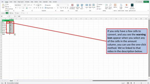
Before jumping into the Paste Special method, it’s worth checking whether you actually need it. If you select a cell in the Amount column and see a small warning icon appear, and you only have a handful of cells to fix, our one-click method is the faster option — click the icon, choose Convert to Number, and you’re done.
We walk through that method step by step in our companion tutorial, linked in the description below. The Paste Special method covered in this guide really shines when you’re converting a large range of cells at once, which is what we’ll cover from here on out.
Step 2: Type The Number 1 In A Blank Cell
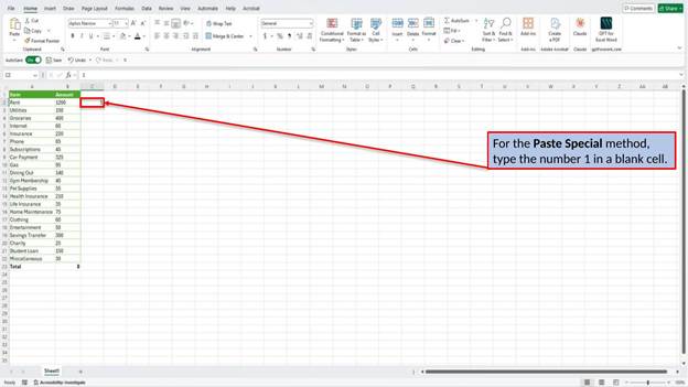
The Paste Special trick works by multiplying every text-stored number by 1. Multiplying forces Excel to treat the result as a genuine number, which converts the text along with it.
To get started, click on any blank cell outside your data range and type the number 1. This acts as a temporary helper cell for the conversion.
Step 3: Copy That Cell
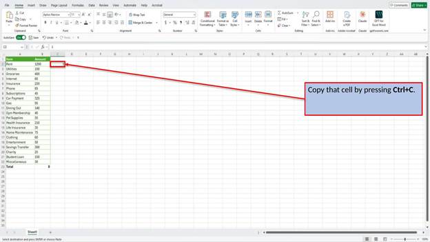
With the number 1 entered, copy that cell by pressing Ctrl+C (or right-click and choose Copy). Copying it places that value on your clipboard, which is what makes the multiply trick possible in the next step.
Step 4: Select The Range Of Cells You Want To Convert
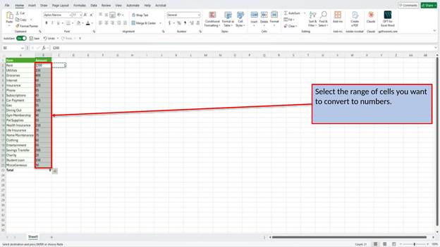
Next, click and drag to select the full range of cells you want to convert — this can be a single column or a much larger block of data, depending on what you’re working with.
Unlike the one-click method, there’s no limit to how many cells you can convert at once, which is what makes this approach so useful for large data sets.
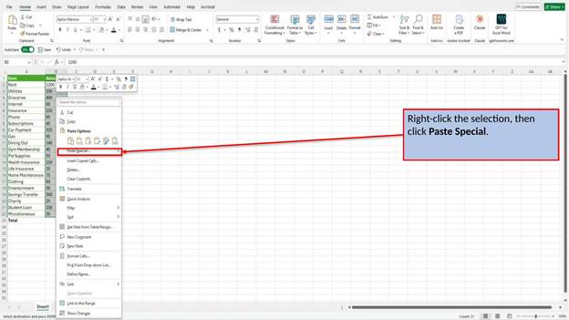
Step 5: Right-Click The Selection And Choose Paste Special
With your range still selected, right-click anywhere inside it and choose Paste Special from the menu. This opens a dialog box with several paste options — we’re only interested in one of them, which we’ll set in the next step.
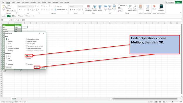
Step 6: Choose Multiply, Then Click OK
In the Paste Special dialog, look for the Operation section and select Multiply, then click OK. This tells Excel to multiply every cell in your selection by the value on your clipboard — the number 1 you copied earlier.
Since multiplying by 1 doesn’t change the value, the only real effect is converting each text-formatted number into a genuine, calculable number.
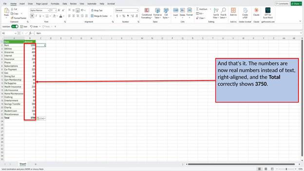
Step 7: Check Your Converted Numbers
Take a look at your data now. The numbers shift to the right side of their cells, which is Excel’s default alignment for actual numbers (text stays left-aligned, a handy way to spot the issue in the future). And the Total row, which showed 0 before, now correctly adds up to 3750.
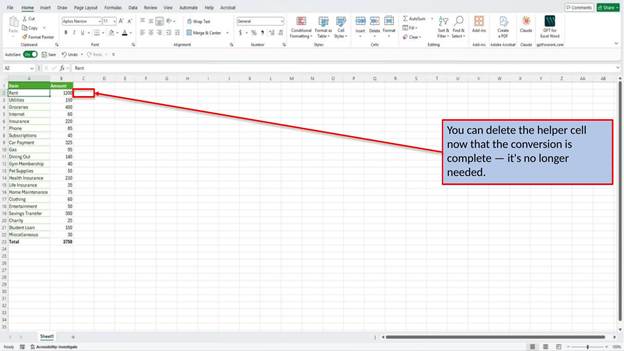
Step 8: Delete The Helper Cell
The last step is just cleanup. Click on the cell where you typed the number 1 and delete it — it was only ever a temporary helper for the conversion, and your data no longer needs it now that every cell holds a real number.
And that’s all it takes to convert text to numbers in Excel using Paste Special. This method isn’t limited to expense lists either — it works just as well on data imported from a CSV file, exported from an accounting system, or pulled from any source that leaves your numbers formatted as text.
The next time you’re staring down a column of numbers that won’t add up right, and there are too many to fix one click at a time, the Paste Special trick will get the whole thing converted in just a few clicks.
Video Tutorial
Download PDF Below