
Click here to view our video tutorial
Click here to download our PDF tutorial
Duplicate entries have a way of sneaking into even the most carefully kept spreadsheets. Maybe you merged two contact lists, imported data from a form that let people submit twice, or simply copied and pasted a row without noticing it was already there. However it happens, the result is the same: a list with repeated names, emails, or other entries that make your data harder to trust and messier to work with.
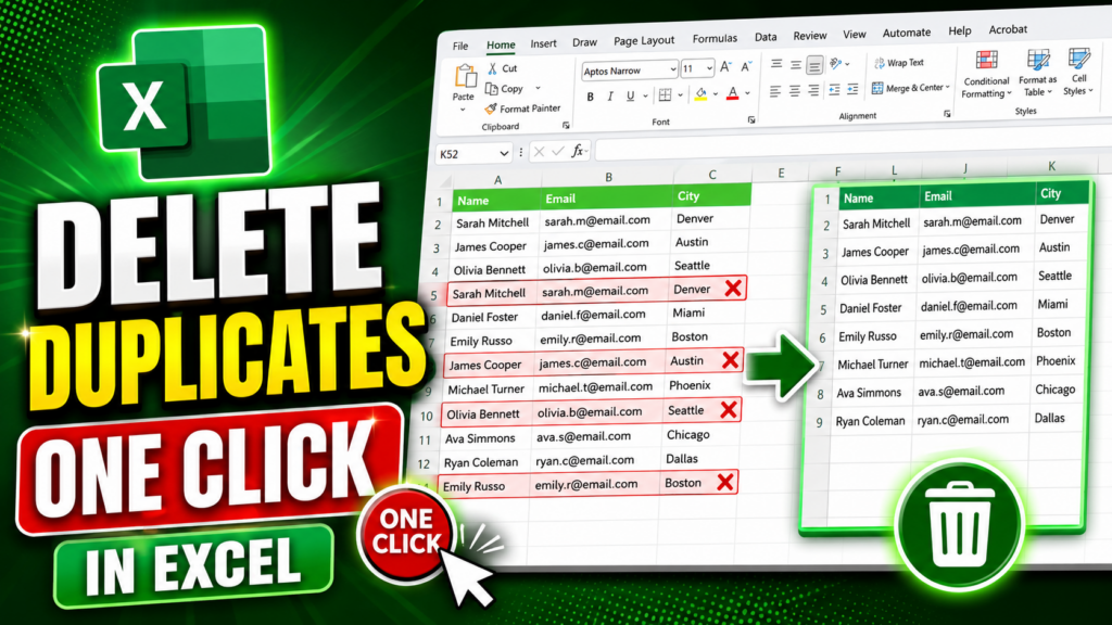
Scrolling through row by row to spot repeats is slow and easy to get wrong, especially on a longer list. Fortunately, Excel has a built-in tool made specifically for this called Remove Duplicates. There’s no formula to write and no manual comparison required. You simply tell Excel where to look, and it finds and removes the repeated entries for you.
In this guide, we’ll walk through exactly how to use Remove Duplicates, starting with a list that has a few repeated names and ending with a clean list containing only unique rows, all done in just a few clicks.
Getting to Know Your Starting Data
Before we get into the steps, take a look at the list we’re starting with. It has a Name column, an Email column, and a City column, and if you look closely, a few entries appear more than once: Sarah Mitchell, James Cooper, Olivia Bennett, and Emily Russo each show up twice. This is a very common situation. It happens any time a list gets merged, imported, or re-entered by hand, and it’s exactly the kind of cleanup Remove Duplicates was built to handle.
Step 1: Select a Cell In Your Data
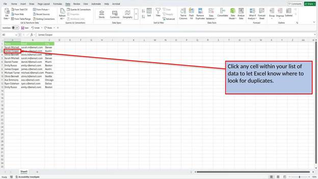
Click any single cell within your list of data. You don’t need to select the whole range yourself, just click anywhere inside it. This tells Excel where your data lives so it knows exactly which rows and columns to check when it looks for duplicates.
Step 2: Open the Data Tab and Click Remove Duplicates
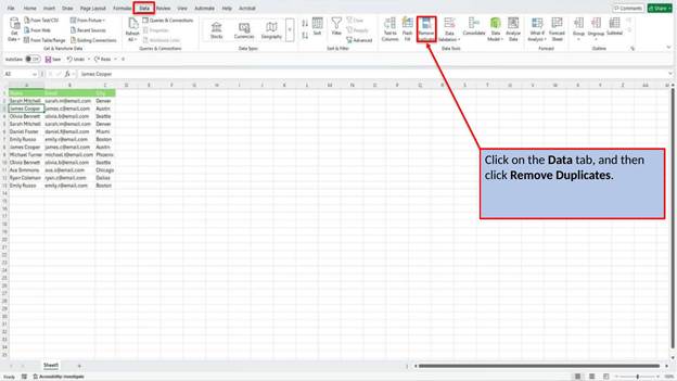
With a cell selected inside your list, click on the Data tab in the ribbon at the top of Excel. In the Data Tools group, you’ll find a button labeled Remove Duplicates. Click it, and Excel opens a dialog box where you’ll confirm exactly how it should check your list.
Step 3: Confirm Your Columns and Click OK
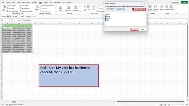
The Remove Duplicates dialog lists every column in your data and lets you choose which ones to check for repeated values. Make sure My data has headers is checked so Excel treats your top row as column titles instead of data to compare. With everything selected the way you want it, click OK to run the check.
Step 4: Review the Confirmation Message
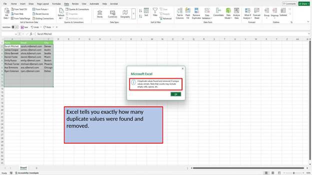
As soon as you click OK, Excel shows you a message telling you exactly how many duplicate values it found and removed, along with how many unique rows remain. This is a handy way to confirm the cleanup worked the way you expected before you move on.
Step 5: Check Your Cleaned-Up List
Take a look at your list now. Every duplicate row is gone, leaving only unique entries behind. Sarah Mitchell, James Cooper, Olivia Bennett, and Emily Russo each appear just once now, and the rest of your list is untouched.
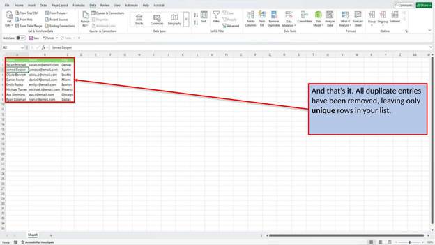
And that’s all it takes to remove duplicate entries from a list in Excel. Remove Duplicates isn’t limited to names and emails either; it works just as well on order numbers, invoice records, product lists, or any other data where repeated rows are throwing off your results. The next time your list starts looking a little too familiar, skip the manual scan and let Excel’s Remove Duplicates tool do the work for you.
Video Tutorial
Download PDF Below