
Last updated: July 26, 2026
Quick Answer: The most valuable spreadsheet formulas for everyday work cover five categories: math and aggregation (SUM, AVERAGE, COUNT), logic (IF, AND, OR), lookup (VLOOKUP, XLOOKUP, INDEX/MATCH), text handling (CONCATENATE, LEFT, TRIM), and date/time (TODAY, DATEDIF). Mastering these 25 core equations in Excel and Google Sheets covers roughly 90% of real business tasks, from budgeting to reporting to data cleanup.
Key Takeaways
- SUM, IF, and VLOOKUP are the three formulas that deliver the most immediate value for beginners.
- Excel and Google Sheets share nearly identical syntax for all 25 formulas covered here, with a few noted exceptions.
- SUMIFS is almost always better than SUMIF because it handles multiple conditions without extra effort.
- Nesting formulas (for example, IF inside VLOOKUP) is the fastest way to build powerful, compact logic.
- The most common formula mistakes are mismatched data types, missing dollar signs in absolute references, and extra spaces in lookup values.
- Beginners can get productive with the top 10 formulas in a weekend; full mastery of all 25 takes 4-6 weeks of regular use.
- Google Sheets has a few exclusive functions (IMPORTRANGE, GOOGLEFINANCE) that Excel doesn’t offer natively.

What Are the Most Important Spreadsheet Formulas to Learn First
The 10 highest-priority formulas for everyday spreadsheet work are SUM, AVERAGE, COUNT/COUNTA, IF, VLOOKUP (or XLOOKUP), SUMIF/SUMIFS, COUNTIF/COUNTIFS, CONCATENATE (or the & operator), TODAY, and IFERROR. These cover budgeting, data lookup, conditional logic, and error handling, the four pillars of most office tasks.
Here’s a quick-reference formula toolbox organized by task category:
| Category | Formula | What It Does |
|---|---|---|
| Math | SUM | Adds a range of numbers |
| Math | AVERAGE | Returns the mean of a range |
| Math | ROUND | Rounds to a set number of decimals |
| Count | COUNT | Counts cells with numbers |
| Count | COUNTA | Counts non-empty cells |
| Count | COUNTIF | Counts cells meeting one condition |
| Count | COUNTIFS | Counts cells meeting multiple conditions |
| Logic | IF | Returns one value if true, another if false |
| Logic | AND / OR | Tests multiple conditions together |
| Logic | IFERROR | Catches errors and shows a fallback value |
| Lookup | VLOOKUP | Finds a value in a table by row |
| Lookup | XLOOKUP | Modern, flexible replacement for VLOOKUP |
| Lookup | INDEX/MATCH | Looks up values in any direction |
| Lookup | HLOOKUP | Finds a value in a table by column |
| Conditional Math | SUMIF | Sums cells meeting one condition |
| Conditional Math | SUMIFS | Sums cells meeting multiple conditions |
| Conditional Math | AVERAGEIF | Averages cells meeting one condition |
| Text | CONCATENATE / & |
Joins text from multiple cells |
| Text | LEFT / RIGHT / MID | Extracts part of a text string |
| Text | TRIM | Removes extra spaces |
| Text | UPPER / LOWER | Changes text case |
| Text | LEN | Returns the length of a text string |
| Date | TODAY | Returns today’s date |
| Date | DATEDIF | Calculates difference between two dates |
| Date | NETWORKDAYS | Counts working days between two dates |
Difference Between Excel and Google Sheets Formulas
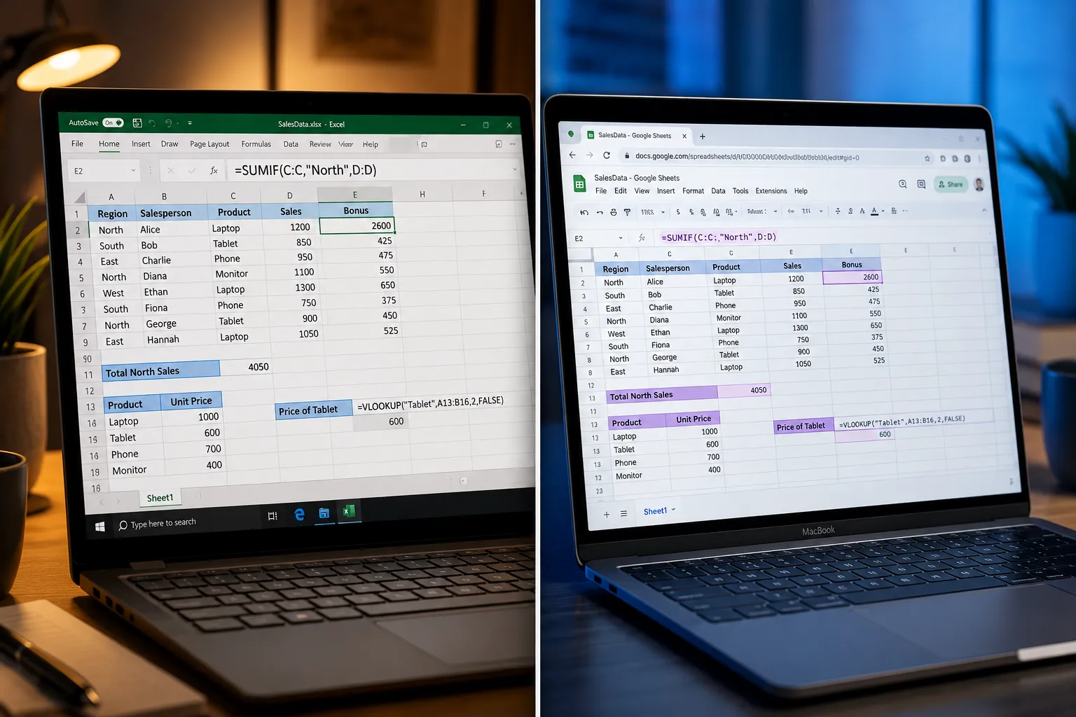
For all 25 formulas in this guide, the syntax is identical between Excel and Google Sheets. Both use the same function names, the same argument order, and the same comma separators (in English-language versions). The practical differences are minor but worth knowing.
Key differences to watch for:
- XLOOKUP is available in Excel 365 and Google Sheets, but not in older Excel versions (2016 or earlier).
- IMPORTRANGE exists only in Google Sheets, it pulls data from another spreadsheet file.
- GOOGLEFINANCE is a Google Sheets-only function for pulling live stock prices.
- Array formulas work differently: Google Sheets uses
ARRAYFORMULA()as a wrapper; Excel uses Ctrl+Shift+Enter or the newer dynamic array syntax. - Decimal separators may differ by locale, some regions use semicolons instead of commas inside formulas.
For a deeper breakdown of where the two platforms diverge, see Spreadsheet Formulas in Google Sheets vs Excel: Key Syntax Differences, Missing Functions, and How to Translate Your Skills.
How to Use VLOOKUP in Excel vs Google Sheets
VLOOKUP finds a value in the leftmost column of a table and returns a value from a specified column to the right. The syntax is identical in both platforms: =VLOOKUP(lookup_value, table_array, col_index_num, [range_lookup]).
Mini use-case (inventory tracking): You have a product list in columns A, C (ID, Name, Price). To find the price for product ID “P102”:
<code>=VLOOKUP("P102", A2:C100, 3, FALSE)
</code>
The FALSE argument forces an exact match, always use it unless you specifically need approximate matching.
VLOOKUP vs XLOOKUP: XLOOKUP is the modern replacement. It searches in any direction, handles missing values more gracefully, and doesn’t break when you insert columns. If your version supports it, use XLOOKUP instead:
<code>=XLOOKUP("P102", A2:A100, C2:C100, "Not found")
</code>
Common mistake: VLOOKUP can only look to the right. If the column you want is to the left of the lookup column, use INDEX/MATCH or XLOOKUP instead.
Best Spreadsheet Formulas for Beginners
Beginners should start with five formulas before anything else: SUM, AVERAGE, IF, COUNTIF, and IFERROR. These five handle the most common tasks and teach the core concepts (ranges, conditions, error handling) that make every other formula easier to learn.
Start here, beginner formula cheat sheet:
=SUM(A2:A50), adds up a column of numbers instantly=AVERAGE(B2:B20), finds the mean of a score or sales column=IF(C2>100, "Over budget", "OK"), flags cells based on a condition=COUNTIF(D2:D50, "Pending"), counts how many tasks are still pending=IFERROR(VLOOKUP(E2,A:B,2,FALSE), "Not found"), prevents ugly#N/Aerrors
💡 Pro tip for beginners: Learn how to insert a formula in Excel for an entire column early, it saves hours of copy-pasting.
What Formulas Do You Need for Budgeting and Expense Tracking
For budgeting and expense tracking, the five most useful formulas are SUMIFS, AVERAGEIF, IF, ROUND, and TODAY. Together they let you total spending by category, flag over-budget items, and keep date-stamped records automatically.
Budget formula toolkit:
=SUMIFS(C2:C100, B2:B100, "Food", A2:A100, ">="&DATE(2026,1,1)), total food spending in 2026=AVERAGEIF(B2:B100, "Travel", C2:C100), average travel expense per transaction=IF(D2>E2, "Over budget", "On track"), status flag comparing actual vs. planned=ROUND(SUM(C2:C50)*0.15, 2), calculates a 15% tax estimate, rounded to cents=TODAY(), auto-fills today’s date in a log entry
For a ready-to-use starting point, check out this monthly food budget template built in Excel 365.
How to Write IF Statements in Spreadsheets
An IF statement returns one result when a condition is true and a different result when it’s false. The syntax is =IF(logical_test, value_if_true, value_if_false) and it works identically in Excel and Google Sheets.
Simple example:
<code>=IF(B2>=60, "Pass", "Fail")
</code>
Nested IF (multiple conditions):
<code>=IF(B2>=90, "A", IF(B2>=75, "B", IF(B2>=60, "C", "F")))
</code>
Using AND/OR inside IF:
<code>=IF(AND(B2>50, C2="Approved"), "Process", "Hold")
</code>
Common mistake: Nesting more than 3-4 IF statements gets hard to read and debug. When you have 5+ conditions, switch to IFS (available in both platforms) or a VLOOKUP against a reference table instead.
For a full walkthrough of logical tests, see Excel IF Statements Made Simple: How to Build Smart Logical Tests.
SUMIF vs SUMIFS: Which One Should You Use
Use SUMIFS by default. SUMIFS handles both single and multiple conditions, while SUMIF only handles one. The syntax is slightly different but SUMIFS is strictly more capable, there’s no reason to use SUMIF unless you’re working in a very old spreadsheet system.
SUMIF (one condition):
<code>=SUMIF(B2:B100, "Marketing", C2:C100)
</code>
SUMIFS (multiple conditions):
<code>=SUMIFS(C2:C100, B2:B100, "Marketing", D2:D100, "Q1")
</code>
Note the argument order flips: in SUMIFS, the sum range comes first. That’s the most common source of errors when switching between the two.
Common Mistakes People Make With Spreadsheet Formulas
The five most frequent formula errors in everyday spreadsheet work are: using relative references when absolute references are needed, looking up text that has hidden spaces, mismatching data types (number stored as text), forgetting to lock ranges in SUMIFS, and circular references.
Quick fixes:
- Missing
$signs: Use F4 (Windows) or Cmd+T (Mac) to toggle absolute references.$A$1stays fixed when copied;A1shifts. - Hidden spaces: Wrap lookup values in
TRIM(),=VLOOKUP(TRIM(A2), ...), to remove invisible leading/trailing spaces. - Numbers stored as text: Multiply by 1 or use
VALUE()to convert:=VALUE(A2)*B2. - Circular reference: A formula that refers to its own cell. Excel and Google Sheets both flag this, check the formula bar for the cell pointing back to itself.
How to Combine Multiple Formulas Together
Nesting formulas means placing one formula inside another as an argument. This is how spreadsheet power users build compact, reusable logic without helper columns.
Three practical nesting patterns:
IFERROR + VLOOKUP, graceful error handling:
=IFERROR(VLOOKUP(A2, Sheet2!A:B, 2, FALSE), "Missing")IF + AND, multi-condition logic:
=IF(AND(B2>0, C2="Active"), B2*0.1, 0)SUMIFS + DATE, dynamic date-range totals:
=SUMIFS(C:C, A:A, ">="&DATE(2026,1,1), A:A, "<="&TODAY())
For more on building reusable calculation blocks, see Spreadsheet Equations for Real Analytics: How to Build Reusable Calculation Blocks in Excel and Google Sheets.
Spreadsheet Formulas for Data Analysis and Reporting
For data analysis and reporting tasks, the highest-value formulas are COUNTIFS, SUMIFS, AVERAGEIF, RANK, LARGE/SMALL, and TEXT. These let you build summary dashboards, rank performers, and format numbers for clean reports, all without leaving the spreadsheet.
Reporting formula examples:
=RANK(B2, B$2:B$50, 0), ranks a sales rep from highest to lowest=LARGE(C2:C50, 3), returns the 3rd highest value in a dataset=TEXT(TODAY(), "MMMM DD, YYYY"), formats a date as “July 26, 2026” for report headers=COUNTIFS(D2:D100, "Closed", E2:E100, ">="&DATE(2026,7,1)), counts closed deals in July 2026
For advanced users who want to push spreadsheets further into database territory, Spreadsheet Formulas for Advanced Users: High-Impact Techniques to Make Excel Work Like a Lightweight Database covers the next level.
What Formulas Work in Google Sheets But Not Excel
Three Google Sheets-exclusive functions stand out: IMPORTRANGE, GOOGLEFINANCE, and SPARKLINE (though Excel has its own Sparklines feature, the formula-based syntax differs). QUERY is also Google Sheets-only and lets you run SQL-style queries on a range.
=IMPORTRANGE("spreadsheet_url", "Sheet1!A1:C100"), pulls live data from another Google Sheets file=GOOGLEFINANCE("GOOG", "price"), returns the current stock price=QUERY(A1:D100, "SELECT A, SUM(D) WHERE B='Sales' GROUP BY A"), aggregates data with SQL-style syntax
Excel users can achieve similar cross-file data pulling with Power Query, but it’s not a single-cell formula.
How Long Does It Take to Master Spreadsheet Formulas
Most people become productive with the top 10 formulas in one focused weekend (roughly 6-8 hours of practice). Comfortable mastery of all 25 core formulas takes 4-6 weeks when practiced on real work tasks daily. Full fluency, including nested formulas, array logic, and data analysis patterns, typically develops over 3-6 months of regular use.
A realistic learning path:
- Days 1-2: SUM, AVERAGE, COUNT, IF, IFERROR
- Week 1-2: VLOOKUP/XLOOKUP, SUMIFS, COUNTIFS, CONCATENATE, TODAY
- Week 3-4: INDEX/MATCH, AVERAGEIF, TEXT, TRIM, LEFT/RIGHT/MID
- Month 2: RANK, LARGE/SMALL, NETWORKDAYS, DATEDIF, nested formulas
- Month 3+: Array formulas, QUERY (Sheets), dynamic arrays (Excel)
If you want to accelerate the process, how to learn MS Excel in 24 hours offers a structured crash-course approach.
Do You Need to Learn All 25 Formulas, or Just Some
No, most people only need 10-15 formulas for their specific job. The full list of 25 gives complete coverage, but the right subset depends on what you actually do.
Choose based on your role:
- Finance/budgeting: SUM, SUMIFS, AVERAGEIF, IF, ROUND, TODAY, NETWORKDAYS
- Sales/reporting: COUNTIFS, RANK, LARGE, VLOOKUP/XLOOKUP, TEXT, IFERROR
- HR/admin: DATEDIF, NETWORKDAYS, COUNTIF, CONCATENATE, TRIM, IF
- Data analysis: INDEX/MATCH, SUMIFS, COUNTIFS, LARGE/SMALL, QUERY (Sheets)
- Students: SUM, AVERAGE, IF, COUNT, ROUND, CONCATENATE
🎯 Decision rule: Start with the 5 beginner formulas. Add formulas only when a real task demands them. Learning in context is faster and stickier than memorizing a full list upfront.
Also worth noting: keyboard shortcuts dramatically speed up formula entry. The Excel Shortcut Keys master list organized by task is a practical companion to formula practice.
FAQ
Q: What is the single most useful spreadsheet formula for a beginner? SUM. It’s the most universally needed, teaches the concept of ranges, and works identically in every spreadsheet application.
Q: Can I use the same formula syntax in Excel on Mac vs Windows? Yes, for all 25 formulas covered here the syntax is identical. The only differences are keyboard shortcuts for entering array formulas and some locale-based separator characters (commas vs semicolons).
Q: What’s the difference between COUNTIF and COUNTIFS? COUNTIF handles one condition; COUNTIFS handles multiple. Like SUMIF vs SUMIFS, always use COUNTIFS, it works for single conditions too and is strictly more flexible.
Q: Why does VLOOKUP return #N/A even when the value exists? Usually because of extra spaces (fix with TRIM), a number stored as text (fix with VALUE), or a case-sensitivity issue. Wrap the lookup value in TRIM() as a first debugging step.
Q: What is IFERROR and when should I use it?
IFERROR wraps any formula and returns a custom value if that formula produces an error. Use it whenever you’re doing lookups or division to prevent ugly error codes from showing in reports: =IFERROR(your_formula, "").
Q: Is XLOOKUP available in Google Sheets? Yes, as of 2023 Google Sheets supports XLOOKUP. It works the same way as in Excel 365.
Q: What does the dollar sign ($) do in a formula like $A$1?
It creates an absolute reference, locking that cell address so it doesn’t shift when the formula is copied to other cells. $A$1 locks both column and row; $A1 locks only the column; A$1 locks only the row.
Q: How do I calculate the number of days between two dates?
Use =DATEDIF(start_date, end_date, "D") for total days, or =NETWORKDAYS(start_date, end_date) to count only working days. For years between dates, use "Y" as the third argument in DATEDIF.
Q: Are there formulas that help clean messy imported data? Yes, TRIM (removes extra spaces), CLEAN (removes non-printable characters), UPPER/LOWER/PROPER (standardizes case), and VALUE (converts text-formatted numbers) are the core data-cleaning formulas. For more, see Excel Text Functions: How to Extract, Combine, and Clean Text.
Conclusion
Mastering Spreadsheet Formulas for Everyday Work: 25 Core Equations You Should Master in Excel and Google Sheets doesn’t require memorizing everything at once. The practical path is to start with five formulas, apply them to real tasks, and expand from there based on what your work actually demands.
Actionable next steps:
- This week: Practice SUM, IF, COUNTIF, IFERROR, and VLOOKUP on a real dataset from your job.
- Next week: Add SUMIFS, AVERAGEIF, CONCATENATE, TODAY, and TRIM.
- This month: Build one working dashboard or budget tracker using at least 8 of the 25 formulas.
- Ongoing: When a task feels repetitive, ask “is there a formula for this?”, there almost always is.
The formulas in this guide work in 2026 across Excel 365, Excel for Mac, and the current version of Google Sheets. The syntax won’t change significantly, so the time spent learning them now pays off for years.