
Last updated: June 21, 2026
Quick Answer: To calculate total cost in Excel, multiply quantity by unit price using
=B2*C2for each line item, then sum all results with=SUM(D2:D10). For a single-step approach, use=SUMPRODUCT(B2:B10,C2:C10)to multiply and sum an entire range at once. These formulas work in all modern Excel versions.
Key Takeaways
- The core formula for a line-item total is
=Quantity * Unit Price(e.g.,=B2*C2) [3] - Use
=SUM(D2:D10)to add all line totals into one grand total =SUMPRODUCT(B2:B10,C2:C10)calculates the grand total in a single formula without a helper column [8]=SUMIFlets you calculate total cost for a specific category or product- Always start every Excel formula with an
=sign — without it, Excel treats the entry as plain text - Lock cell references with
$(e.g.,$C$2) when copying formulas across rows to avoid errors - Format your total cost cells as Currency or Accounting for clean, readable output
- Named ranges (e.g.,
Quantity,UnitPrice) make formulas easier to read and audit
Why Excel Is the Go-To Tool for Cost Calculations
Excel handles cost calculations reliably because its formula engine updates every total automatically when any input changes. Whether you’re tracking grocery expenses, managing a project budget, or building a pricing sheet for a small business, knowing how to calculate total cost in Excel formula saves time and reduces manual errors. [9]
The approach scales from a five-row shopping list to a thousand-row inventory without changing the formula logic — only the cell range changes.
Setting Up Your Spreadsheet Before Writing Any Formula
A clean layout is the foundation of accurate cost calculations. Before typing a single formula, set up these four columns:
| Column | Label | Example Data |
|---|---|---|
| A | Item | Office Chair |
| B | Quantity | 4 |
| C | Unit Price | 125.00 |
| D | Total Cost | (formula goes here) |
Quick setup tips:
- Put headers in Row 1 so your data starts in Row 2 — this keeps formulas consistent
- Format column C as Currency before entering prices (right-click → Format Cells → Currency)
- Freeze the top row so headers stay visible as data grows — see this guide on how to freeze the top row and first column simultaneously in Excel for a fast way to do it
- Use Excel shortcuts to expand all columns so no data gets cut off visually
Common mistake: Entering prices as text (e.g., “$125”) instead of plain numbers. Excel can’t multiply text. Always enter raw numbers and let cell formatting add the currency symbol.
How to Calculate Total Cost in Excel Formula: The Basic Method
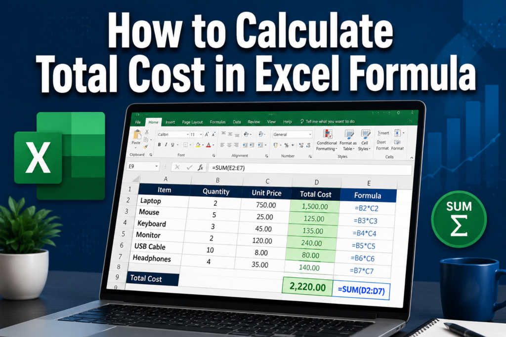
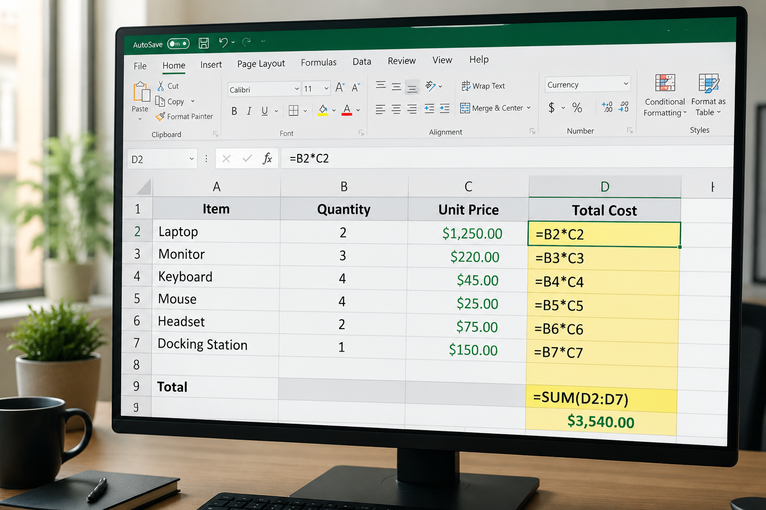
The simplest way to calculate total cost per line item is a multiplication formula. In cell D2, type:
<code>=B2*C2
</code>
This multiplies the quantity in B2 by the unit price in C2 and returns the total cost for that row. [3]
To apply it to all rows:
- Click cell D2 (where you just entered the formula)
- Hover over the bottom-right corner of the cell until you see a small + (the fill handle)
- Double-click or drag down to copy the formula through all data rows
Excel automatically adjusts the row numbers — D3 gets =B3*C3, D4 gets =B4*C4, and so on.
Then add a grand total in the row below your data:
<code>=SUM(D2:D10)
</code>
Adjust D10 to match your last data row. This sums every line-item total into one number. [9]
Choose this method if: You want to see each line-item total separately AND a grand total. It’s the most transparent layout for invoices, budgets, or any document others need to review.
How to Calculate Total Cost in Excel Formula Using SUMPRODUCT
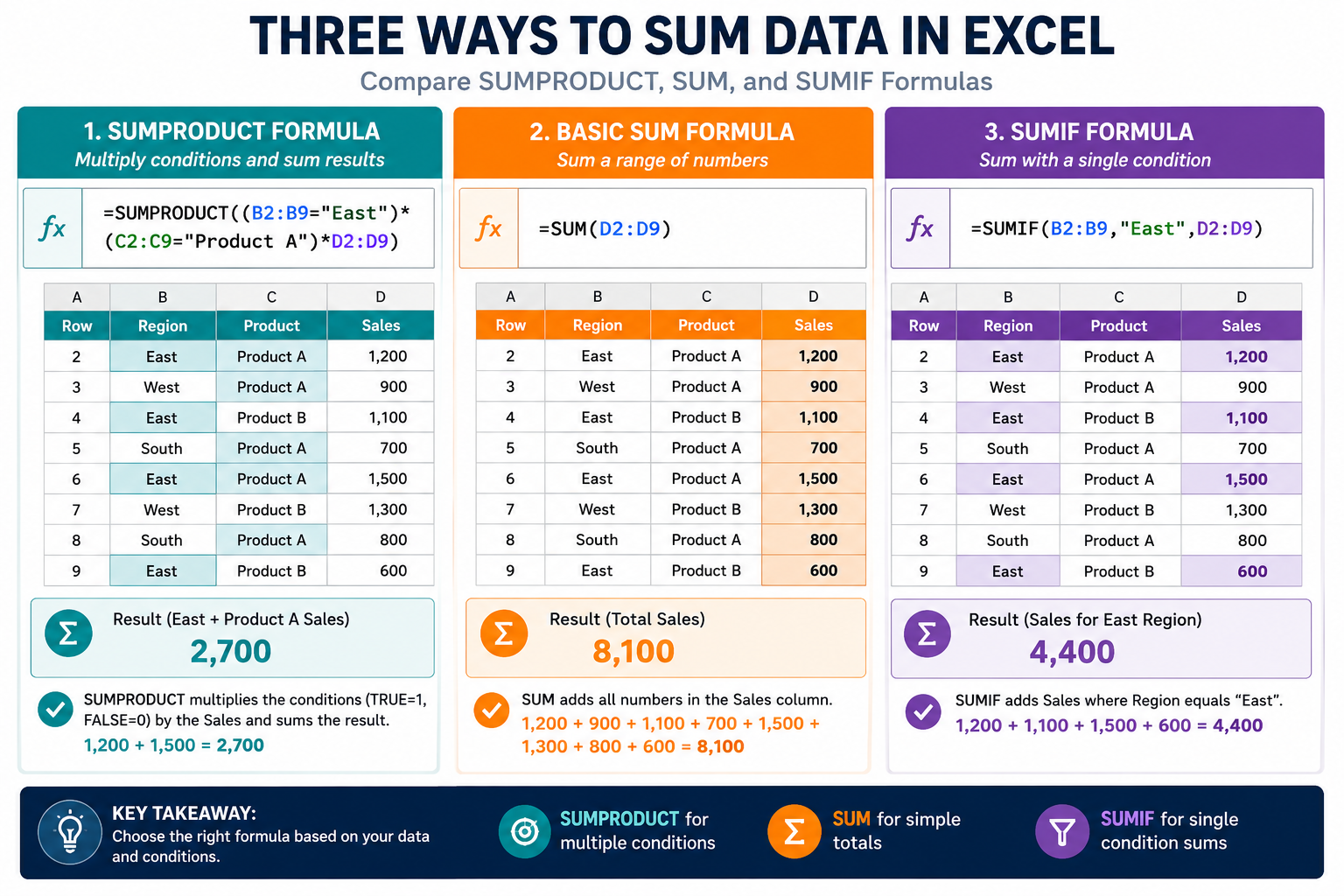
SUMPRODUCT calculates the grand total cost in one formula, skipping the helper column entirely. [8]
<code>=SUMPRODUCT(B2:B10, C2:C10)
</code>
This formula multiplies each quantity by its matching unit price, then adds all the results together automatically.
When to use SUMPRODUCT vs. the basic method:
| Situation | Best Formula |
|---|---|
| Need to see each row’s total | =B2*C2 per row + =SUM() |
| Want a single grand total cell | =SUMPRODUCT(B2:B10,C2:C10) |
| Calculating cost for one category | =SUMIF() (see next section) |
| Working with very large datasets | =SUMPRODUCT() (faster to set up) |
Edge case: If your quantity or price column contains blank cells, SUMPRODUCT treats them as zero and still returns a correct result. Empty rows won’t cause errors.
Using SUMIF to Calculate Total Cost for a Specific Category
Sometimes you need the total cost for just one product type or department. SUMIF handles this cleanly.
Scenario: Column A lists product categories, column D holds line totals. To get the total cost for “Electronics” only:
<code>=SUMIF(A2:A10, "Electronics", D2:D10)
</code>
Or, if you want to multiply and filter at the same time, combine SUMPRODUCT with a condition:
<code>=SUMPRODUCT((A2:A10="Electronics") * B2:B10 * C2:C10)
</code>
This is useful for cost breakdowns by vendor, department, or product line without needing a pivot table.
For more ways to add numbers by row, check out this resource on how to add numbers in rows in Excel with a formula.
How to Handle Tax, Discounts, and Markups in Your Total Cost Formula
Real-world cost calculations rarely stop at quantity times price. Here’s how to extend the formula for common adjustments:
Adding sales tax (e.g., 8%):
<code>=SUMPRODUCT(B2:B10, C2:C10) * 1.08
</code>
Applying a discount (e.g., 10% off):
<code>=SUMPRODUCT(B2:B10, C2:C10) * 0.90
</code>
Adding tax after a discount:
<code>=SUMPRODUCT(B2:B10, C2:C10) * 0.90 * 1.08
</code>
Best practice: Store the tax rate and discount percentage in dedicated cells (e.g., E1 for tax, E2 for discount), then reference them in the formula:
<code>=SUMPRODUCT(B2:B10, C2:C10) * (1 - E2) * (1 + E1)
</code>
This way, changing the tax rate updates every total automatically — no formula editing needed.
To protect these rate cells from accidental edits, see the guide on how to lock specific cells in Excel.
Rounding Your Total Cost Results
Financial totals often need rounding to two decimal places to avoid values like $47.999999. Use ROUND to fix this:
<code>=ROUND(SUMPRODUCT(B2:B10, C2:C10), 2)
</code>
The second argument (2) sets the number of decimal places. Use 0 for whole-dollar rounding.
For rounding up specifically (useful for billing or inventory), ROUNDUP works the same way:
<code>=ROUNDUP(SUMPRODUCT(B2:B10, C2:C10), 2)
</code>
Learn more about how to use the ROUNDUP function in Excel for additional rounding scenarios.
Making Your Cost Tracker Easier to Read
A formula is only as useful as the spreadsheet around it. A few formatting steps make cost data much easier to scan:
- Alternate row colors so the eye can track across wide rows — here’s how to apply color to alternate rows using conditional formatting
- Highlight cells that exceed a budget threshold using conditional formatting traffic lights to flag cost overruns at a glance
- Add a chart to visualize cost distribution — the Ten Tips for Excel Charts series shows how to build one in seconds with Alt + F1
For a ready-made starting point, the monthly food budget template for Excel 365 already includes total cost formulas you can adapt.
Common Errors and How to Fix Them
| Error | Likely Cause | Fix |
|---|---|---|
#VALUE! |
A cell contains text instead of a number | Check for currency symbols typed into cells; use Format Cells instead |
#REF! |
A referenced cell was deleted | Recheck the formula range after deleting rows |
| Formula shows as text | Missing = at the start |
Click the cell, press F2, add = at the beginning |
| Wrong total after copying | Relative references shifted incorrectly | Use $ to lock references that shouldn’t change |
| Total is zero | Range doesn’t match data rows | Expand the SUM or SUMPRODUCT range to include all data rows |
FAQ
Q: What is the basic Excel formula to calculate total cost?
The basic formula is =Quantity * Unit Price, for example =B2*C2. Add =SUM(D2:D10) below all rows to get the grand total.
Q: How do I calculate total cost for an entire column in Excel?
Use =SUM(D2:D100) where D2:D100 covers your total cost column. Excel ignores empty cells in the range.
Q: Can I calculate total cost without a helper column?
Yes. =SUMPRODUCT(B2:B10, C2:C10) multiplies and sums in one step, so no separate Total Cost column is needed.
Q: How do I add tax to a total cost formula in Excel?
Multiply the result by (1 + tax rate). For 8% tax: =SUMPRODUCT(B2:B10,C2:C10)*1.08. Store the rate in a cell and reference it for easy updates.
Q: Why does my total cost formula show #VALUE!? A cell in the referenced range contains text or a symbol (like a typed “$”) instead of a plain number. Remove the symbol from the cell and apply Currency formatting instead.
Q: What’s the difference between SUM and SUMPRODUCT for total cost?
SUM adds a list of pre-calculated totals. SUMPRODUCT multiplies two ranges together and sums the results in one step — it’s more efficient when you haven’t calculated individual row totals yet.
Q: How do I calculate total cost for only one product type?
Use =SUMIF(A2:A10,"ProductName",D2:D10) where column A holds category names and column D holds line totals.
Q: How do I round a total cost to two decimal places?
Wrap the formula: =ROUND(SUMPRODUCT(B2:B10,C2:C10),2). The 2 sets the decimal places.
Q: Does SUMPRODUCT work if some cells are blank? Yes. Blank cells are treated as zero, so the formula still returns a correct total without errors.
Q: How do I apply the same total cost formula to 500 rows quickly? Enter the formula in the first row, click the cell, then double-click the fill handle (bottom-right corner). Excel copies the formula down to match the length of adjacent data automatically.
Conclusion
Knowing how to calculate total cost in Excel formula is one of the most practical skills in any spreadsheet toolkit. Start with =B2*C2 for line-item totals and =SUM(D2:D10) for the grand total. When you want a single-cell solution, =SUMPRODUCT(B2:B10,C2:C10) does the job without a helper column. Add ROUND, SUMIF, or tax multipliers as your needs grow.
Actionable next steps:
- Open a blank Excel workbook and build a four-column layout (Item, Quantity, Unit Price, Total Cost) right now
- Enter five sample rows of data and apply
=B2*C2to the Total Cost column - Add a grand total row using
=SUM(D2:D6) - Try replacing the grand total with
=SUMPRODUCT(B2:B6,C2:C6)and confirm the numbers match - Apply currency formatting and alternate row colors to make the sheet presentation-ready
Once the basics feel natural, explore the home inventory template for Excel 365 — it’s a real-world example of these formulas in action.
References
[3] Creating An Excel Formula To Calculate Total Cost – https://learn.microsoft.com/en-us/answers/questions/1372480/creating-an-excel-formula-to-calculate-total-cost
[8] Excel Formula Calculate Total Cost – https://codepal.ai/excel-formula-generator/query/wAYvTTe7/excel-formula-calculate-total-cost
[9] Excel Tutorial Find Total Cost – https://excel-dashboards.com/blogs/blog/excel-tutorial-find-total-cost