
Click here to view our video tutorial.
Click here to download our PDF tutorial.
Hello, and welcome to Mark’s Excel Tips. In this tutorial, I will show you how to get a cell, in Excel to change color based on its value. Let’s get started.
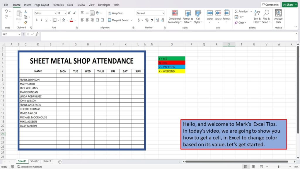
Here we have an attendance roster used to document each employee’s attendance.

The first thing that we did is to determine what colors we wanted based on the values that we enter into each cell.

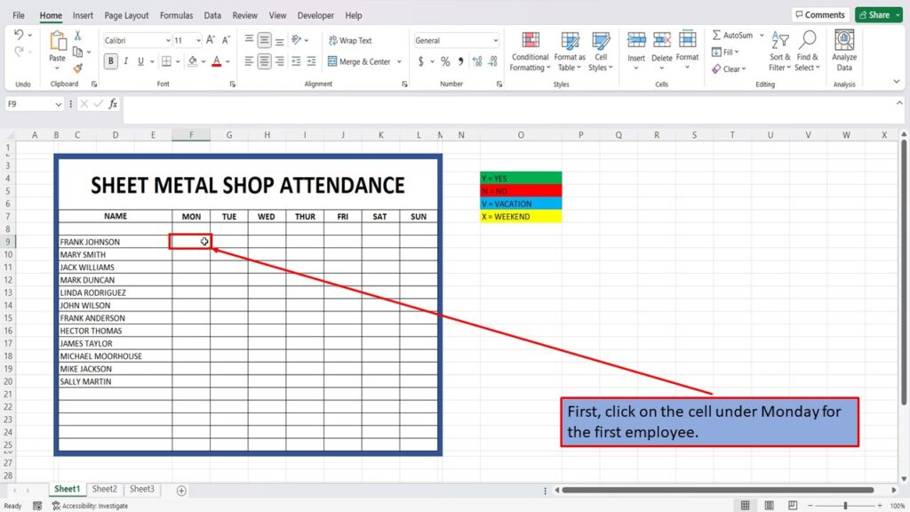
First, click on the cell under Monday for the first employee.
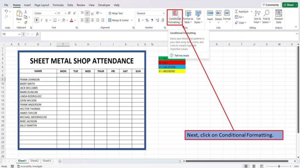
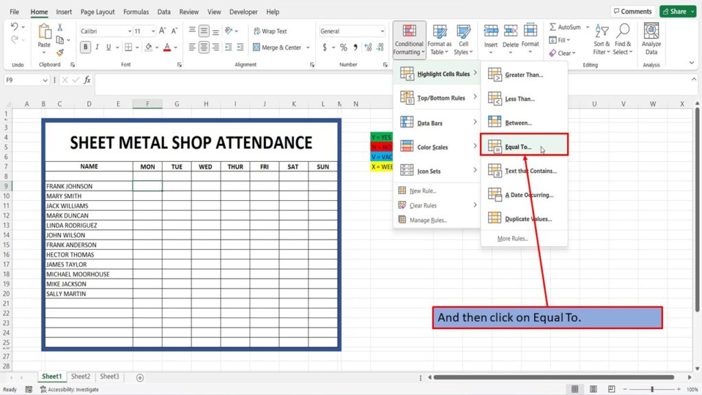
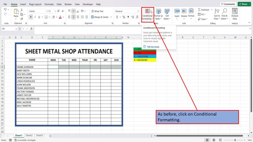
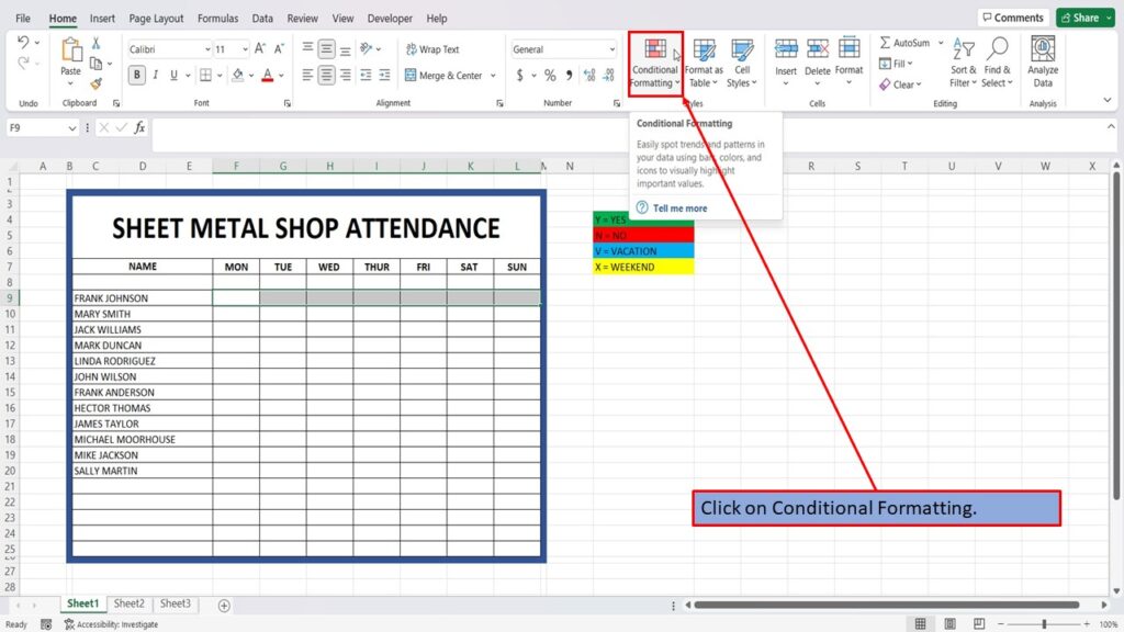
Next, click on Conditional Formatting.
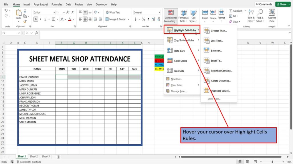
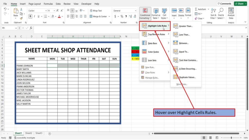
Hover your cursor over Highlight Cells Rules.
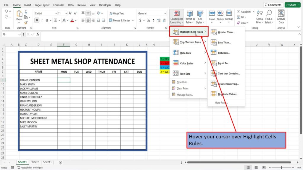
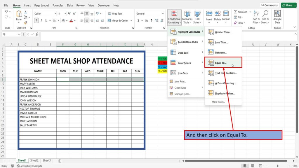
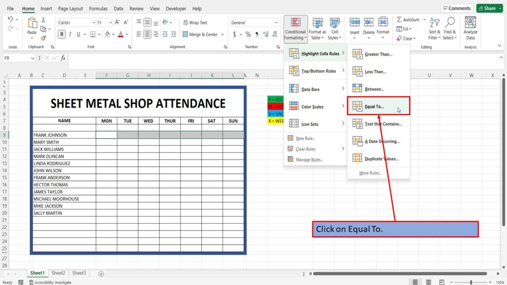
And then click on Equal To.
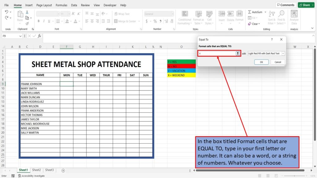
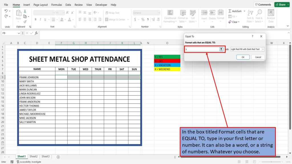
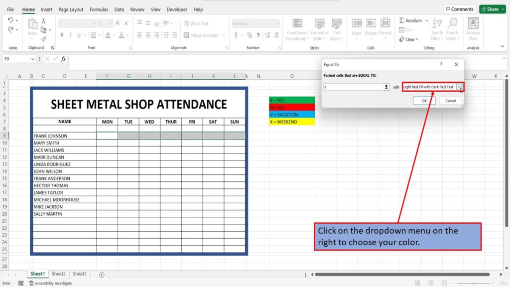
In the box titled Format cells that are EQUAL TO, type in your first letter or number. It can also be a word, or a string of numbers. Whatever you choose.
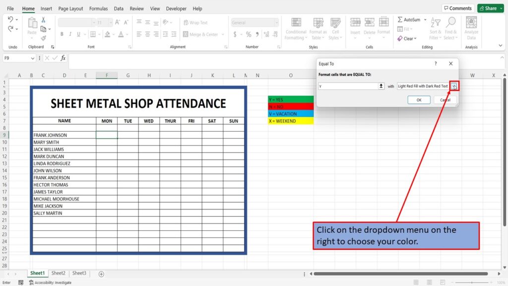
Click on the dropdown menu on the right to choose your color.
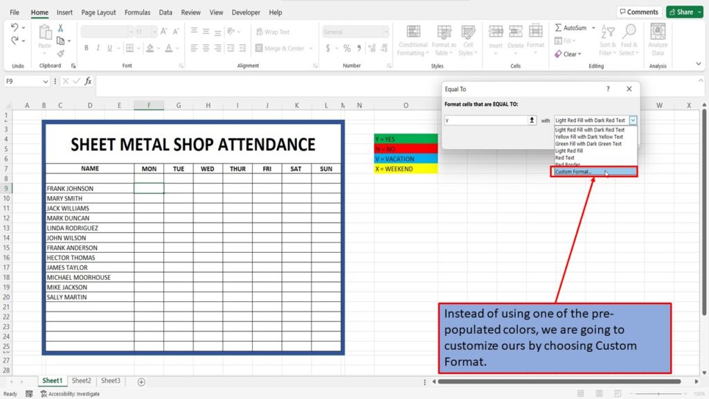
Instead of using one of the pre-populated colors, we are going to customize ours by choosing Custom Format.
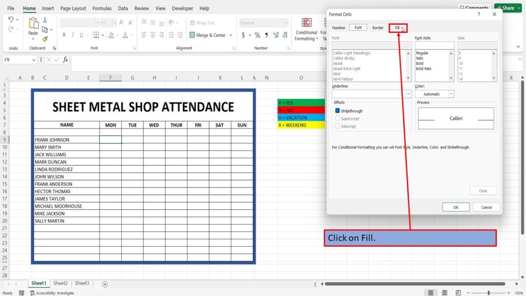
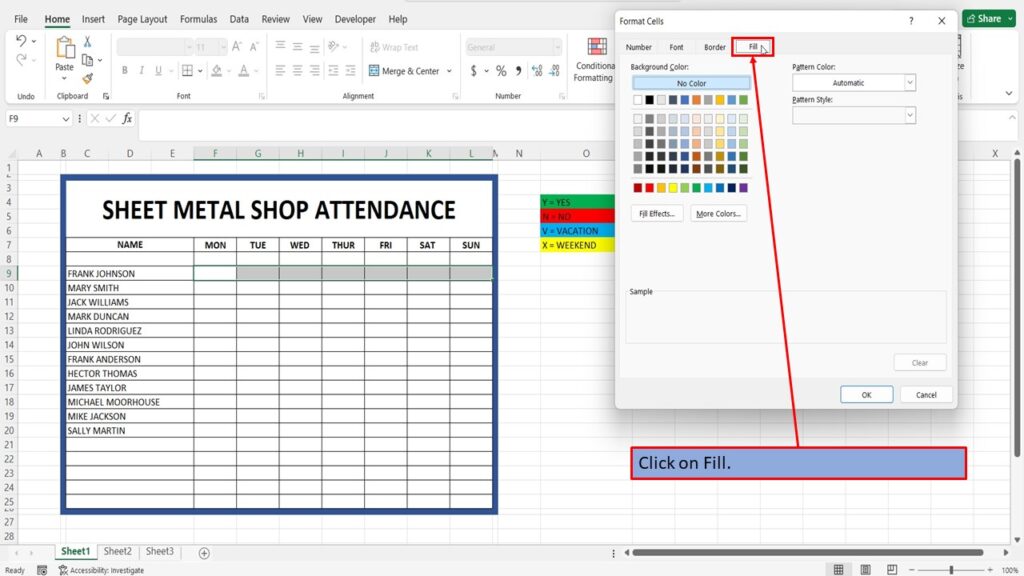
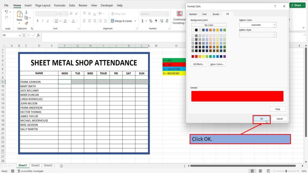
Click on Fill.
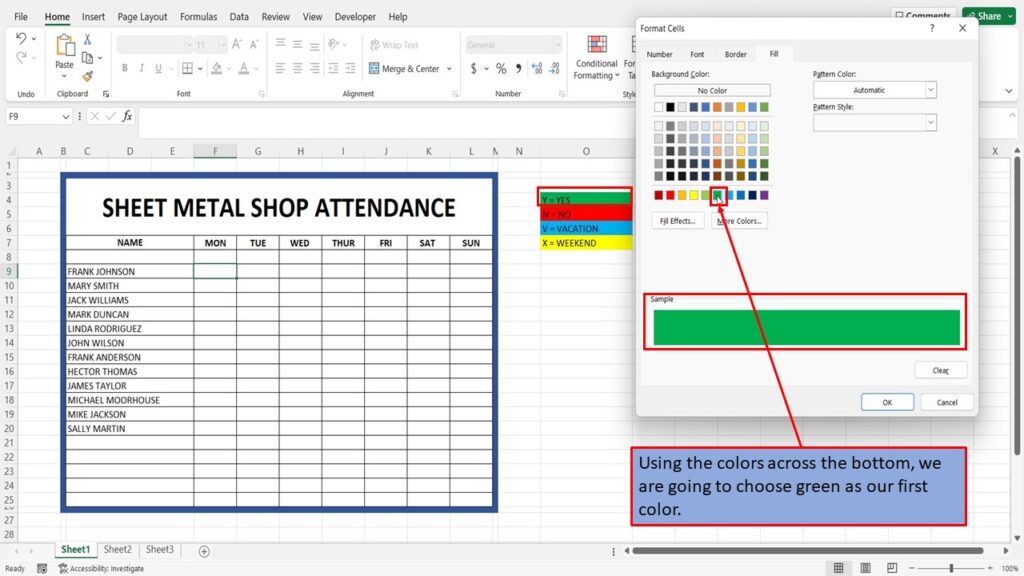
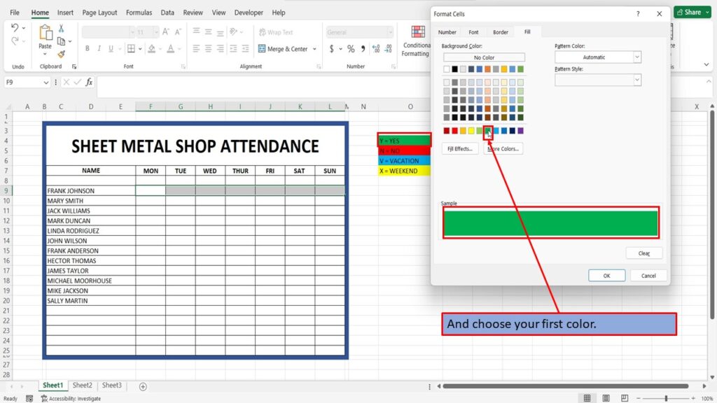
Using the colors across the bottom, we are going to choose green as our first color.
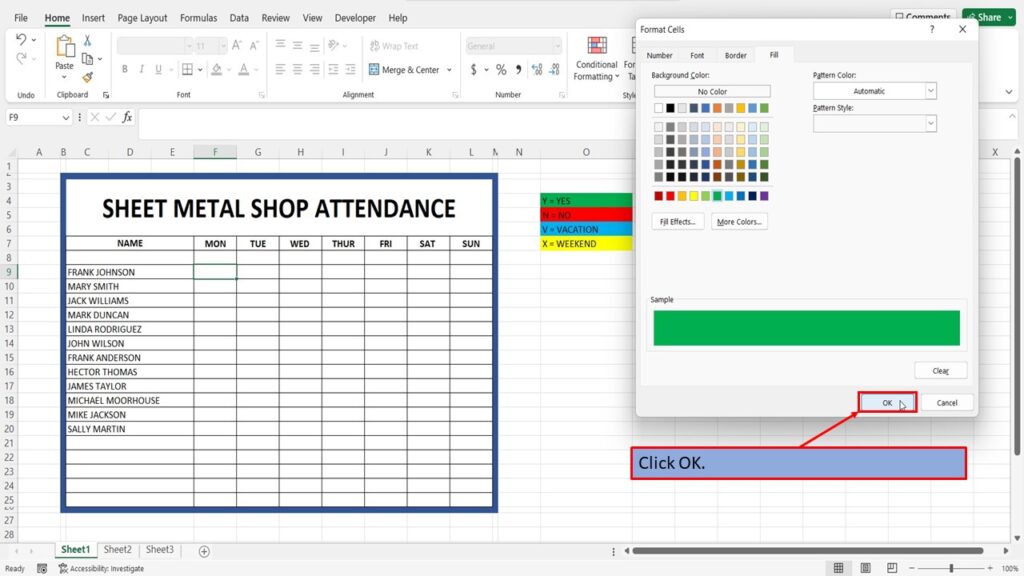
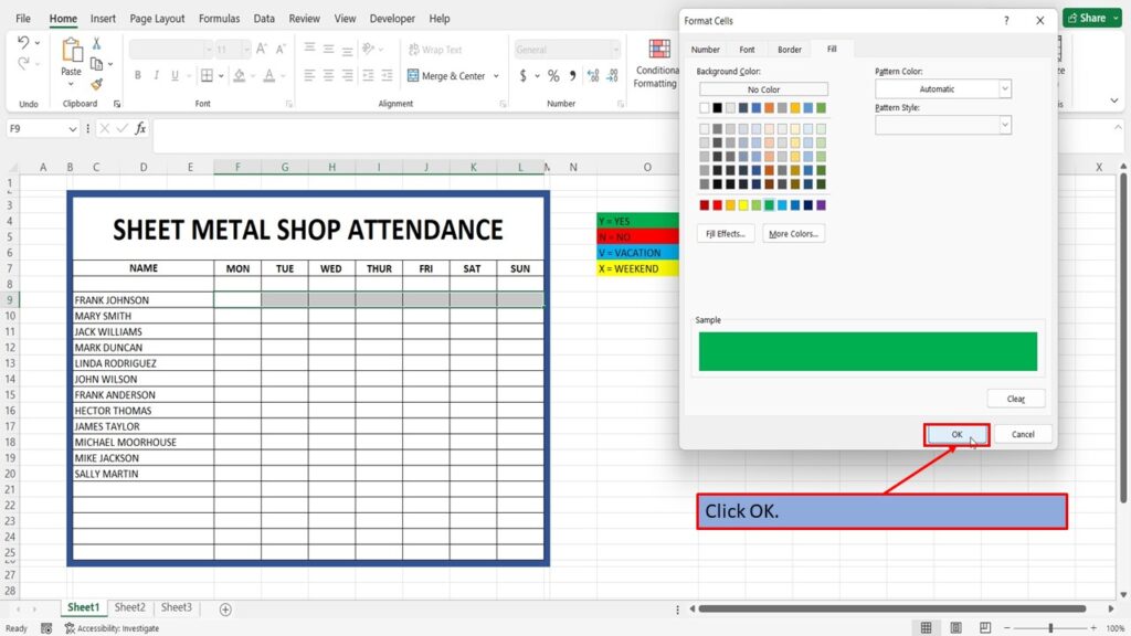
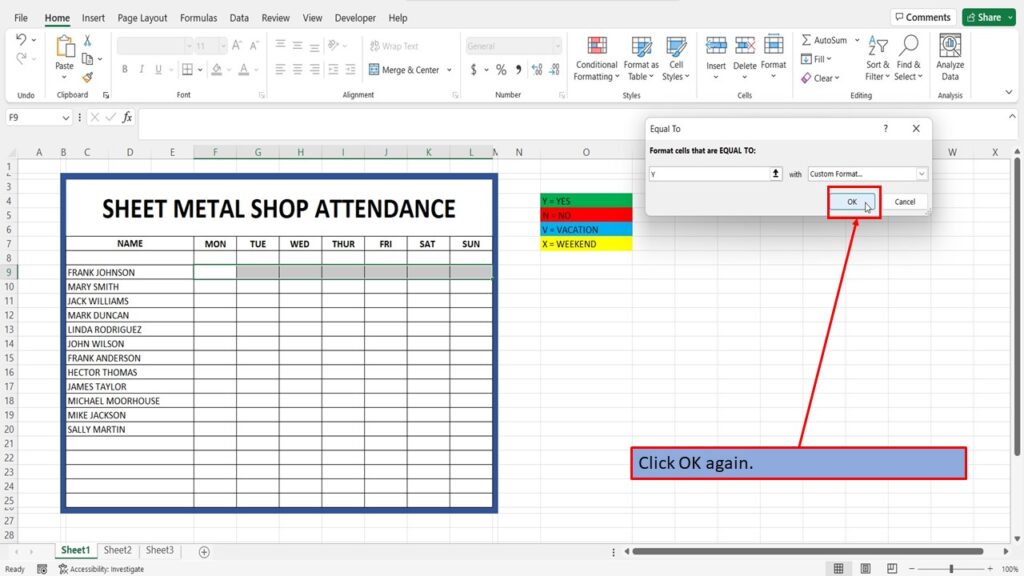
Click OK.
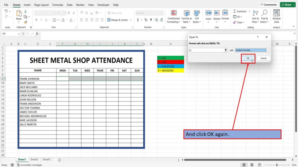
Click OK again.

Now, when you put the letter Y into the cell it automatically turns green.

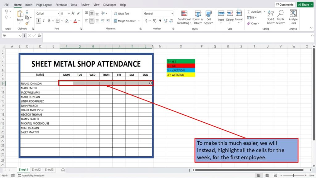
If you were to do each cell this way it would be a lot of work and take a long time to format each and every cell in this workbook.

To make this much easier, we will instead, highlight all the cells for the week, for the first employee.
As before, click on Conditional Formatting.
Hover your cursor over Highlight Cells Rules.
And then click on Equal To.
In the box titled Format cells that are EQUAL TO, type in your first letter or number. It can also be a word, or a string of numbers. Whatever you choose.
Click on the dropdown menu on the right to choose your color.
Click on Custom Format.

Click on Fill.
And choose your first color.
Click OK.
Click OK again.
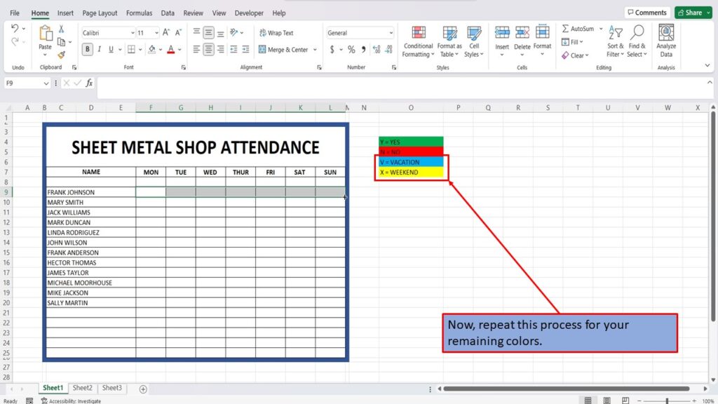
Now, we are going to repeat this same process for the remainder of the colors.

Click on Conditional Formatting.
Hover over Highlight Cells Rules.
Click on Equal To.
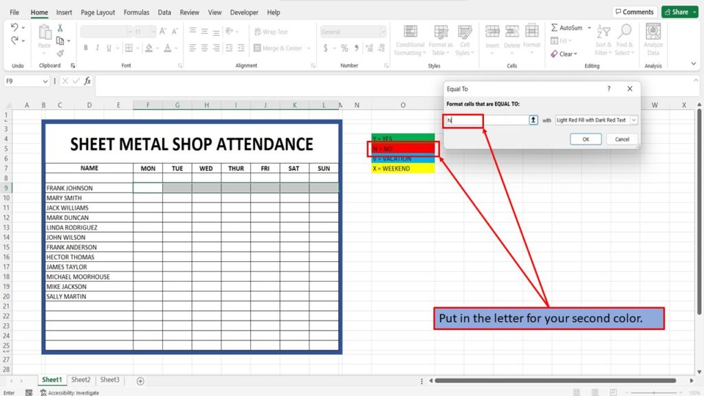
Put in the letter for your second color.
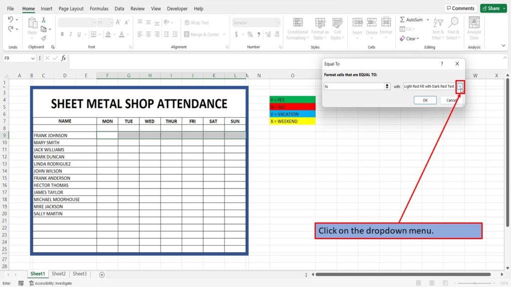
Click on the dropdown menu.
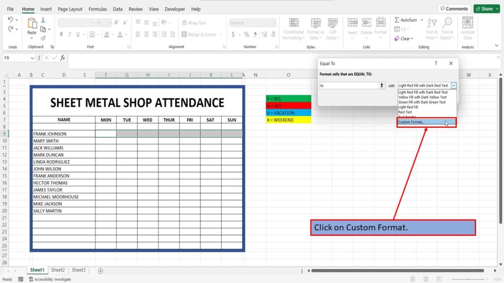
Click on Custom Format.
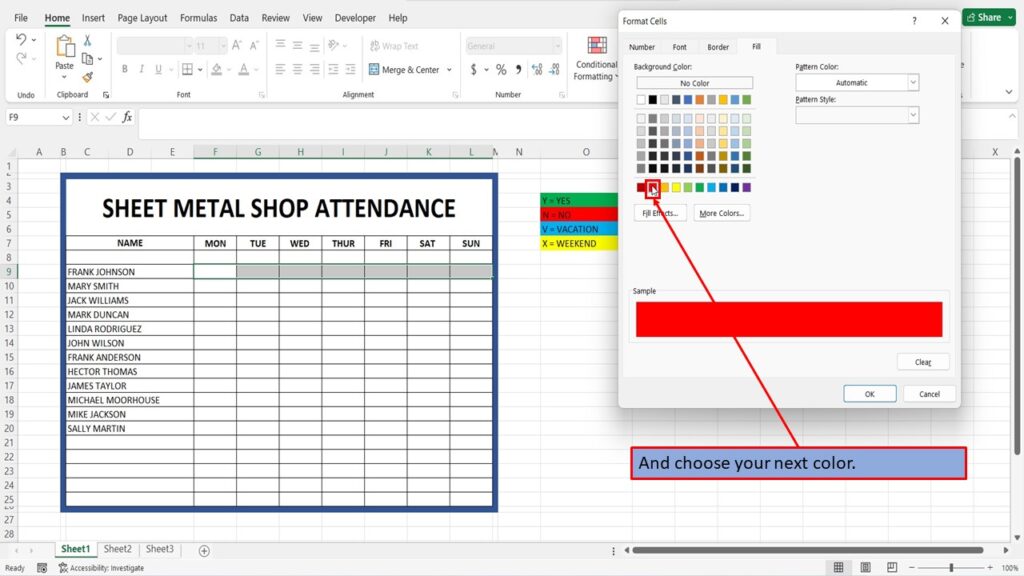
And choose your next color.
Click OK.
And click OK again.
Now, repeat this process for your remaining colors.
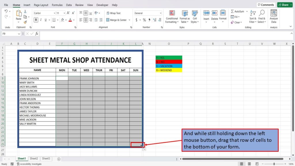
Once you have completed this for all of your colors, left click on the plus sign in the bottom right of the cells that you have highlighted.
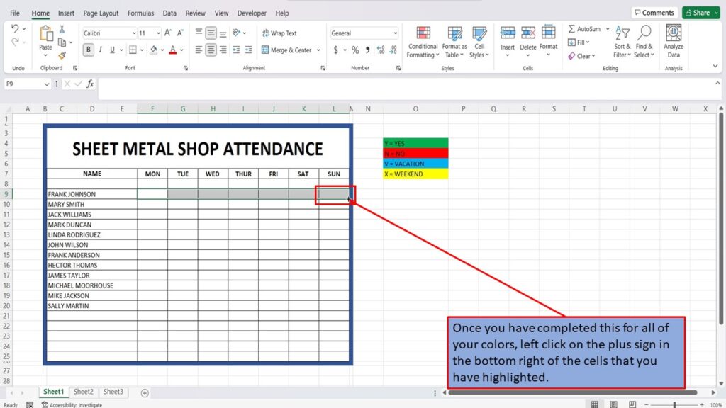
And while still holding down the left mouse button, drag that row of cells to the bottom of your form.
You now have an Excel worksheet where the cells will change color based on that cells input.

View the Video Tutorial.
Download this tutorial in PDF by clicking the Download link below.