how to insert formula in excel for entire column

Last updated: June 7, 2026

Quick Answer: To insert a formula in Excel for an entire column, type your formula in the first cell, then either double-click the fill handle, press Ctrl + D after selecting the range, or use Ctrl + Enter after selecting the whole column. If your data is in an Excel Table, typing the formula once applies it to every row automatically. [1]

Key Takeaways

Double-clicking the fill handle is the fastest method for most datasets — it copies the formula down to the last row of adjacent data automatically.
Ctrl + D fills a formula down a selected range without touching a mouse.
Excel Tables auto-expand formulas to new rows, making them the best choice for growing datasets.
Absolute references (like $A$1) lock a cell so it doesn’t shift when you copy a formula down; relative references (like A1) do shift — and that’s usually what you want.
Ctrl + Enter applies one formula to every selected cell at once, even non-consecutive ones.
Blank cells in a column can stop the fill handle’s auto-detect — use Ctrl + Shift + End to manually select the full range instead.
Array formulas (entered with Ctrl + Shift + Enter in older Excel versions, or dynamic arrays in Excel 365) can handle entire column calculations in a single formula.
Excel Tables and named ranges make formulas easier to read and maintain over time.

What Does Dragging a Formula Down in Excel Actually Do?

When you drag a formula down a column, Excel copies the formula into each new cell and adjusts relative cell references automatically. So if your formula in C2 is =A2*B2, dragging it to C3 makes it =A3*B3, and so on. [1]

This behavior is called relative referencing, and it’s what makes dragging so powerful for column-wide calculations. Excel isn’t just pasting the same formula — it’s recalculating which rows each reference points to based on how far you’ve moved.

Quick example: A sales sheet has quantities in column A and prices in column B. Entering =A2*B2 in C2 and dragging down through C100 gives you a revenue figure for every row — no manual editing needed.

Common mistake: Dragging too far and overwriting data below your dataset. Always check where your data ends before dragging.

How to Copy a Formula to an Entire Column Without Manually Dragging

There are several reliable ways to apply a formula to an entire column without dragging, and each suits a different situation. [1]

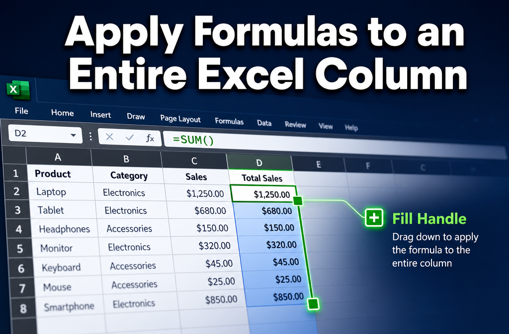
Method 1 — Double-click the fill handle

Enter your formula in the first data cell (e.g., C2).
Click that cell to select it.
Hover over the small green square at the bottom-right corner of the cell (the fill handle).
Double-click it. Excel copies the formula down to match the length of the adjacent data column.

Method 2 — Ctrl + D (Fill Down)

Enter your formula in the top cell.
Select that cell plus all the cells below where you want the formula.
Press Ctrl + D. Done.

Method 3 — Ctrl + Enter (apply to a pre-selected range)

Click the Name Box (top-left, shows the cell address).
Type the range, e.g., C2:C500, and press Enter to select it.
Type your formula directly.
Press Ctrl + Enter instead of just Enter. The formula fills every selected cell at once. [1]

Method 4 — Excel Table (most automatic)

Convert your data range to a table: select any cell in the range, press Ctrl + T.
Type your formula in the first empty cell of a new column.
Press Enter. Excel fills it down the entire column instantly. [1]

For a deeper look at selecting large ranges quickly, see this guide on selecting the entire worksheet in Excel using only shortcut keys.

Is There a Keyboard Shortcut to Apply a Formula to an Entire Column?

Yes. Ctrl + D is the primary shortcut for filling a formula down a selected column range. Ctrl + R does the same thing horizontally (fills right). [1]

For a full-column approach without a mouse:

Use the Name Box to type your range (e.g., D2:D1000).
Press Enter to confirm the selection.
Type your formula.
Press Ctrl + Enter.

This method works well for large datasets where scrolling to find the last row would be slow.

Do Absolute and Relative Cell References Matter When Copying Formulas?

Absolutely — this is one of the most important concepts when learning how to insert a formula in Excel for an entire column. Getting references wrong is the top cause of broken formulas after copying. [1]

Reference Type	Example	What Happens When Copied Down
Relative	`=A2*B2`	Adjusts to `=A3B3`, `=A4B4`, etc.
Absolute	`=$A$2*B2`	`$A$2` stays fixed; only B adjusts
Mixed	`=A$2*B2`	Row locked, column adjusts

When to use absolute references: Any time your formula refers to a fixed value — like a tax rate in cell E1 or a discount percentage in F2. Add a $ before the column letter and row number (e.g., $E$1) to lock it.

Shortcut: Press F4 while your cursor is inside a cell reference in the formula bar to cycle through all four reference types.

For related reading on locking cells, see how to lock specific cells in Excel.

What’s the Fastest Way to Apply a Formula to a Large Dataset?

For large datasets (thousands of rows), the fastest method is the Name Box + Ctrl + Enter approach or converting data to an Excel Table. Dragging manually or even double-clicking the fill handle can be unreliable if there are gaps in adjacent columns.

Step-by-step for large datasets:

Click the Name Box and type the exact range: C2:C50000.
Press Enter to select the range.
Type your formula (e.g., =A2+B2).
Press Ctrl + Enter.

Excel applies the formula to all 49,999 cells in one action. [1]

Performance tip: Avoid applying volatile functions like NOW() or RAND() to entire columns in large files — they recalculate every time the sheet changes and can slow Excel noticeably.

For more formula-building techniques, the formula to add date and time in Excel guide covers useful date-related examples.

Why Are My Excel Cell References Changing When I Copy a Formula?

This is expected behavior — and it’s usually correct. Excel uses relative references by default, so references shift as the formula moves to new rows. [1]

If references are changing when you don’t want them to, the fix is simple: add $ signs to lock the reference.

=A2 becomes =A$2 (locks the row) or =$A$2 (locks both row and column).
Press F4 while editing a reference to toggle between reference types quickly.

Edge case: If you copy a formula sideways (across columns) and the row references shift unexpectedly, check whether you intended relative row references. Copying down shifts rows; copying right shifts columns.

Can I Insert a Formula for Multiple Columns at Once?

Yes. Select a multi-column range before entering your formula, then press Ctrl + Enter. For example, select C2:E100, type =A2*B2, and press Ctrl + Enter — every cell in that range gets the formula with adjusted references.

Alternatively, in an Excel Table, each column is independent, so you’d add a formula to each column separately. But for a block formula across many columns at once, the Ctrl + Enter method is the most direct approach.

Choose this if: You’re building a calculation grid where the same formula logic applies across several adjacent columns simultaneously.

What Happens If I Have Blank Cells When Applying a Formula?

Blank cells in the adjacent column stop the double-click fill handle from auto-detecting the full data range. Excel reads the adjacent column to estimate how far down to fill, and it stops at the first gap it finds.

Workarounds:

Select the full target range manually using the Name Box, then use Ctrl + D or Ctrl + Enter.
Convert the data to an Excel Table — tables ignore gaps in adjacent columns and fill the entire column.
Use Ctrl + Shift + End to select from the current cell to the last used cell in the sheet, then fill down.

Formula behavior in blank source cells: If your formula references a blank cell (e.g., =A5 where A5 is empty), Excel typically returns 0 for numeric formulas or an empty string for text formulas. Wrap with IF(A5="","",your_formula) to suppress unwanted zeros.

How Do I Insert a Formula for Non-Consecutive Cells?

Use Ctrl + Click to select individual non-consecutive cells, type your formula, then press Ctrl + Enter. The formula applies to all selected cells at once, with relative references adjusting for each cell’s position. [1]

This is useful when you need to skip header rows, subtotal rows, or cells with special formatting that shouldn’t be overwritten.

Limitation: Non-consecutive selections can’t be filled with Ctrl + D — that only works on a continuous range. Stick with Ctrl + Enter for scattered cells.

How Do I Fix Broken Formulas After Copying Down a Column?

Broken formulas after copying usually fall into a few categories. Here’s how to diagnose and fix each:

Error	Likely Cause	Fix
`#REF!`	A referenced cell was deleted or the formula moved outside its valid range	Check and correct cell references; use absolute refs if needed
`#VALUE!`	Formula expects a number but found text	Check source data for mixed data types
`#DIV/0!`	Dividing by a blank or zero cell	Wrap with `IFERROR(formula, "")`
`#NAME?`	Formula name misspelled or function not recognized	Check spelling; confirm the function exists in your Excel version

Quick diagnostic: Press Ctrl + ` (backtick) to toggle formula view — you’ll see all formulas in the sheet at once, making it easy to spot where references went wrong.

Also useful: how to round numbers in Excel when formula results need rounding after copying down.

Can I Use Formulas with Different Data Types in the Same Column?

Technically yes, but it creates problems. Excel formulas in a column work most reliably when all cells in the referenced range share the same data type (all numbers, all text, all dates). Mixing types can produce #VALUE! errors or unexpected results.

Best practice: Keep source data clean and consistent. If a column contains both numbers and text, use ISNUMBER() or ISTEXT() checks inside your formula to handle each type separately.

For date-specific formulas, see how to find the difference between two dates in years — a good example of handling date data types correctly in formulas.

Are There Differences Between Excel Versions for Formula Insertion?

The core methods (fill handle, Ctrl + D, Ctrl + Enter) work in all modern Excel versions. The main differences are in advanced formula capabilities:

Excel 365 / Excel 2021+: Dynamic array formulas (like FILTER, SORT, UNIQUE) spill results automatically into a range — no need to copy down manually. One formula in one cell can populate an entire column.
Excel 2019 and earlier: Array formulas require Ctrl + Shift + Enter and don’t spill dynamically.
Excel Tables: Available since Excel 2007; calculated columns work the same across all versions that support tables.
Excel Online: Supports most formula methods but has limited VBA support.

Choose dynamic arrays if you’re on Excel 365 and want a formula that automatically adjusts as your data grows — no copying needed at all.

FAQ

Q: What’s the quickest way to apply a formula to an entire column in Excel? Double-click the fill handle after entering the formula in the first cell. For large or gapped datasets, use the Name Box to select the full range, type the formula, and press Ctrl + Enter.

Q: How do I apply a formula to an entire column without selecting it first? Convert your data to an Excel Table (Ctrl + T). Entering a formula in any cell of a new column automatically fills it down the entire column. [1]

Q: What does Ctrl + D do in Excel? Ctrl + D fills the formula from the top cell of a selected range down into all other selected cells below it. Select the cell with the formula plus the cells below, then press Ctrl + D.

Q: Why does my formula show the same result in every row instead of adjusting? Your cell references are likely absolute (e.g., $A$1). Remove the $ signs to make them relative so they adjust as the formula copies down.

Q: Can I apply a formula to an entire column including millions of rows? Excel supports up to 1,048,576 rows. You can select C2:C1048576 via the Name Box and apply a formula, but doing so on volatile or complex formulas will slow performance significantly. Use Excel Tables or dynamic arrays for efficiency.

Q: How do I stop Excel from auto-filling a formula in a Table column? Go to File > Options > Proofing > AutoCorrect Options > AutoFormat As You Type and uncheck “Fill formulas in tables to create calculated columns.”

Q: What’s the difference between Ctrl + Enter and Ctrl + D? Ctrl + Enter applies the formula you just typed to all pre-selected cells simultaneously. Ctrl + D copies the formula from the top cell of a selection downward. Both achieve similar results, but Ctrl + Enter works without a starting formula already in a cell.

Q: Do formulas in Excel columns update automatically when data changes? Yes, by default Excel recalculates formulas whenever referenced cells change. If formulas aren’t updating, check that calculation is set to Automatic: Formulas tab > Calculation Options > Automatic.

Q: Can I use a formula across an entire column and still add up that column’s results? Yes. Use SUM() or AutoSum on the formula column. For more on summing rows and columns, see how to add up a row of numbers in Excel.

Conclusion

Knowing how to insert a formula in Excel for an entire column is one of those skills that saves hours every week once it clicks. Start with the double-click fill handle for everyday tasks, switch to Ctrl + Enter with a Name Box range for large or gapped data, and convert datasets to Excel Tables when you want formulas to expand automatically as new rows come in.

Actionable next steps:

Open a spreadsheet you use regularly and try converting the data range to an Excel Table.
Practice using F4 to toggle between absolute and relative references — it’ll prevent most copy-paste formula errors.
For complex calculations, explore dynamic array formulas if you’re on Excel 365; they eliminate the need to copy formulas down at all.
Bookmark the keyboard shortcuts: Ctrl + D (fill down), Ctrl + R (fill right), Ctrl + Enter (fill selection), and Ctrl + “ (toggle formula view).

Small habits like these compound quickly into serious Excel efficiency.

References

[1] Use Calculated Columns In An Excel Table – https://support.microsoft.com/en-us/office/use-calculated-columns-in-an-excel-table-873fbac6-7110-4300-8f6f-aafa2ea11ce8