Spreadsheet Equations for Real Analytics: How to Build Reusable Calculation Blocks in Excel and Google Sheets

Last updated: July 12, 2026

Quick Answer: Reusable calculation blocks are self-contained formula modules, named ranges, LAMBDA functions, or structured table references, that you build once and apply across multiple sheets, reports, or projects without rewriting logic. In both Excel and Google Sheets, the core approach is to isolate each calculation (profit margin, cohort retention, cost allocation) into a named, documented unit that pulls from a single source of truth. This saves time, reduces errors, and makes your analytics models far easier to maintain.

Key Takeaways

Named ranges and Excel Tables are the foundation of every reusable formula system, they replace fragile cell references like D4:D200 with readable names like Revenue.
LAMBDA (Excel) and named custom functions (Google Sheets) let you package multi-step logic into a single callable function with no VBA required.
Absolute references ($A$1) lock a formula to a fixed cell; relative references (A1) shift automatically, choosing the right one is critical for analytics templates.
Dynamic array functions like FILTER, UNIQUE, and SEQUENCE (both platforms) make formulas that expand automatically as new data arrives.
Excel’s ARRAYFORMULA equivalent is implicit spill behavior; Google Sheets uses the explicit ARRAYFORMULA() wrapper, the two behave differently in key ways.
A well-organized calculation library uses a dedicated “Config” sheet for constants, a “Calc” sheet for logic blocks, and output sheets for dashboards.
Common mistakes include mixing absolute and relative references incorrectly, hardcoding values inside formulas, and skipping documentation.
When formula complexity exceeds roughly 5 nested functions, VBA (Excel) or Apps Script (Google Sheets) is worth considering.

What Are Reusable Calculation Blocks in Spreadsheets?

A reusable calculation block is a formula or group of formulas that encapsulates one piece of business logic, say, gross margin or 30-day retention, so it can be called or copied anywhere without modification. Think of it like a function in programming: define the logic once, then reuse it with different inputs.

In practice, a calculation block has three parts:

Inputs, cells or named ranges that feed data in (e.g., Revenue, COGS).
Logic, the formula or LAMBDA that processes those inputs.
Output, a cell or spill range that returns the result.

Who benefits most: Analysts who run the same report weekly, finance teams building rolling forecasts, and small business owners tracking KPIs across multiple product lines. If you’re new to formulas in general, the beginner’s guide to writing spreadsheet formulas is a solid starting point before diving into reusable blocks.

Named Ranges vs. Cell References for Analytics Formulas

Named ranges almost always win for analytics work. A formula like =Revenue - COGS is immediately understandable; =D4 - E4 is not, and it breaks the moment someone inserts a column.

Here’s a quick comparison:

Approach	Readability	Maintenance	Risk
Cell reference (`D4:D200`)	Low	High effort	Breaks on insert/delete
Named range (`Revenue`)	High	Low effort	Stays valid after edits
Excel Table column (`Table1[Revenue]`)	High	Automatic	Expands with new rows

How to create a named range:

Excel: Select the cells → Formulas tab → Define Name.
Google Sheets: Select the cells → Data → Named ranges.

Excel Tables (Insert → Table) go one step further: they auto-expand when new rows are added, so a formula referencing SalesData[Amount] always covers every row, no manual range updates needed. For analytics that runs on live data, this is the single most useful habit to build. You can also lock specific cells in Excel to protect input ranges from accidental edits.

What’s the Difference Between Absolute and Relative References in Analytics?

Absolute references ($A$1) stay fixed when a formula is copied; relative references (A1) shift to match the new position. Mixing them up is the most common source of broken analytics templates.

A practical rule:

Use absolute for constants, rate tables, and config values (e.g., =$B$2 for a tax rate).
Use relative for row-by-row calculations that should shift down the column.
Use mixed ($A1 or A$1) when you need to lock only one dimension, common in cross-tab models.

Example, cost allocation across departments:

<code>=C5 * $B$2   ← C5 is the dept spend (relative, shifts per row)
              ← $B$2 is the overhead rate (absolute, stays fixed)
</code>

Copy this formula down 50 rows and it works perfectly. Remove the $ signs and every row uses a different overhead rate, a silent, hard-to-spot error. For a deeper look at logical formula construction, see Excel IF Statements Made Simple.

How to Create Formulas That Work Across Multiple Sheets

Cross-sheet formulas use a sheet reference prefix: SheetName!CellAddress in both Excel and Google Sheets. For reusable analytics, the best pattern is a dedicated “Config” or “Data” sheet that all calculation sheets reference.

Step-by-step setup:

Create a sheet named Config with all constants (tax rates, targets, exchange rates).
Create a sheet named CalcBlocks for your reusable formula modules.
In any output or dashboard sheet, reference: =CalcBlocks!GrossMargin or =Config!TaxRate.
Name the key output cells in CalcBlocks so other sheets can call them by name, not by address.

Edge case: In Google Sheets, cross-file references use IMPORTRANGE(). This is powerful but adds a dependency, if the source file is deleted or access is revoked, all downstream formulas break. For critical analytics, keep everything in one workbook where possible.

How to Build a Template for Recurring Analytics Calculations

A good analytics template separates inputs, logic, and outputs into distinct sheets, and uses named ranges or LAMBDA functions to make each calculation block portable. [2]

Here’s a minimal three-sheet structure that works for profit models, cohort analysis, and cost allocations:

Sheet 1: Config

Company name, reporting period, tax rate, discount rate
All values are named (e.g., TaxRate, DiscountRate)

Sheet 2: CalcBlocks

Each row or section is one calculation module
Column A: block name (e.g., “Gross Margin %”)
Column B: formula (e.g., =(Revenue - COGS) / Revenue)
Column C: description/notes

Sheet 3: Dashboard

Pulls results from CalcBlocks using named references
No raw formulas here, only display logic

💡 Pro tip: Protect the Config and CalcBlocks sheets so collaborators can only edit the input data, not the formula logic. This is one of the most overlooked steps in shared analytics workbooks.

For a practical example of how templates are structured end-to-end, the Project Timeline Template for Excel shows clean sheet organization principles you can adapt.

Excel Array Formulas vs. Google Sheets ARRAYFORMULA for Analytics

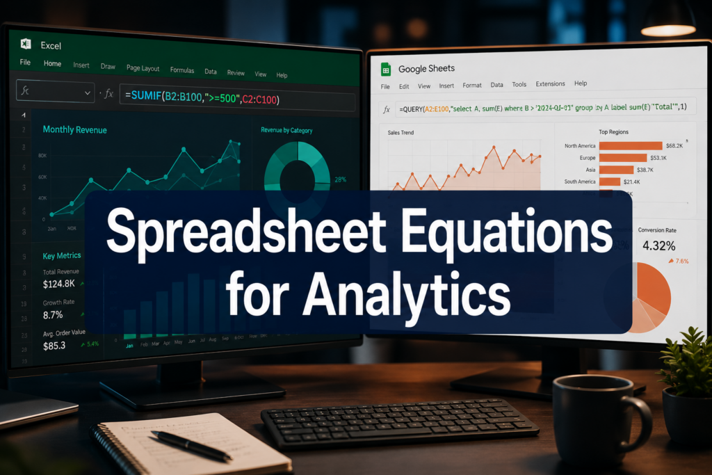
Excel (Microsoft 365) uses implicit spill arrays, dynamic array functions like FILTER, SORT, and UNIQUE automatically output to a range without any wrapper. Google Sheets requires the explicit ARRAYFORMULA() function to extend most formulas across a range. [6]

Key differences:

Excel dynamic arrays spill results automatically. Write =FILTER(SalesData, SalesData[Region]="West") and it fills as many rows as needed.
Google Sheets ARRAYFORMULA wraps a formula to apply it to a whole column: =ARRAYFORMULA(IF(A2:A100>0, B2:B100*C2:C100, 0)).
Performance: Excel handles large spill arrays faster on local machines. Google Sheets ARRAYFORMULA can slow down on 50,000+ row datasets, consider QUERY() for large-scale filtering instead.

LAMBDA in Excel (Microsoft 365): LAMBDA lets you define a custom function directly in the Name Manager, no VBA needed. For example:

<code>=LAMBDA(revenue, cogs, (revenue - cogs) / revenue)
</code>

Name this GrossMarginPct and call it anywhere: =GrossMarginPct(D2, E2). [6]

Google Sheets named functions (available since 2023) work similarly: go to Data → Named functions, define your formula with parameter names, and reuse it across the file. [6]

How to Create Dynamic Formulas That Adjust to New Data Automatically

Dynamic formulas use structured table references, OFFSET, or dynamic array functions so they automatically include new rows without manual range updates. [3]

The three most reliable approaches:

Excel Tables, Any formula referencing Table1[Column] expands instantly when a new row is added. This is the simplest and most reliable method.
OFFSET + COUNTA, =OFFSET($A$1, 0, 0, COUNTA($A:$A), 1) creates a range that grows with data. Useful in older Excel versions without dynamic arrays.
Dynamic array functions, =UNIQUE(A:A) or =FILTER(A:A, B:B="Active") always reflect the current data state.

Common mistake: Using a hardcoded range like A2:A500 and assuming it’s “big enough.” When data exceeds row 500, the formula silently misses rows. Always use a Table or a dynamic range instead. [4]

For hands-on practice with Excel’s calculation capabilities, how to use Excel to calculate walks through the core mechanics step by step.

Best Practices for Organizing Complex Spreadsheet Equations

The biggest organizational wins come from three habits: naming everything, documenting inline, and keeping logic out of display sheets. [2]

Naming conventions that work:

Use prefixes: cfg_ for config values, calc_ for intermediate results, out_ for final outputs.
Avoid spaces in names, use underscores (Gross_Margin_Pct not Gross Margin %).
Keep names under 25 characters for readability in formula bars.

Documentation inside the spreadsheet:

Add a Notes column next to every formula block explaining what it calculates and what inputs it expects.
Use cell comments for non-obvious logic.
Keep a “Changelog” tab that logs what was modified and when.

Structural rules:

One formula per cell, never chain 8 nested functions when you can break them into intermediate steps.
Constants never live inside formulas. =D2 * 0.21 is fragile; =D2 * TaxRate is maintainable.
Color-code input cells (yellow), calculated cells (white/no fill), and output cells (blue or green) so collaborators know what to touch.

Common Mistakes When Building Reusable Spreadsheet Formulas

The most damaging mistakes are hardcoded values, broken references after sheet restructuring, and formulas that silently return wrong results instead of errors. [4]

Watch out for these specifically:

Hardcoded numbers inside formulas, =A2*1.08 should be =A2*(1+TaxRate). When the rate changes, one cell update fixes everything.
Circular references, a formula that refers back to its own cell. Excel and Sheets warn about these, but they can slip in when copying blocks between sheets.
Volatile functions overused, NOW(), TODAY(), RAND(), and OFFSET() recalculate on every change. In large models, this tanks performance. Cache results where possible.
VLOOKUP instead of XLOOKUP/INDEX-MATCH, VLOOKUP breaks when columns are inserted to the left of the lookup column. XLOOKUP and INDEX/MATCH are column-order independent. [4]
Forgetting to lock the formula sheet, leaving calculation blocks editable means a collaborator can accidentally overwrite a LAMBDA definition.

How to Debug Formulas That Aren’t Calculating Correctly

Start by isolating the broken section: evaluate the formula step by step, check that all named ranges resolve correctly, and verify that data types match what the formula expects.

Excel debugging toolkit:

Formulas → Evaluate Formula, steps through each part of a nested formula one click at a time.
Trace Precedents / Trace Dependents, draws arrows showing which cells feed into or depend on the selected cell.
F9 key, highlight any part of a formula in the formula bar and press F9 to see its current value.

Google Sheets debugging:

Use helper columns to break a complex formula into parts and check each intermediate result.
IFERROR(formula, "CHECK THIS") surfaces hidden errors in large ranges.
The Named functions panel shows if a custom function definition has a syntax error.

Most common root causes:

Text stored as numbers (check with ISNUMBER())
Extra spaces in lookup values (fix with TRIM())
Date format mismatches between sheets
A named range pointing to a deleted or moved sheet

When Should You Use VBA or Apps Script Instead of Formulas?

Switch to VBA (Excel) or Apps Script (Google Sheets) when your logic requires loops, conditional branching across multiple sheets, external data connections, or automation that runs on a schedule. Formulas are stateless, they can’t remember previous values or trigger actions. Scripts can.

Choose formulas if:

The calculation is a single-pass transformation of existing data.
The result needs to update live as data changes.
The file will be shared with users who don’t have scripting access.

Choose VBA/Apps Script if:

You need to generate reports automatically at a set time.
The process involves copying, formatting, or emailing output.
The formula would require more than 5 levels of nesting to express.

For most analytics use cases, profit models, cohort retention, KPI dashboards, formulas with LAMBDA or named functions handle everything without scripting overhead. [6]

How to Version Control and Maintain Spreadsheet Equation Libraries

Version control for spreadsheets is manual by default, but a consistent naming and backup system prevents the “which version is final?” problem that kills most analytics projects.

Practical version control steps:

Keep a Changelog sheet inside every analytics workbook with columns: Date, Change Description, Modified By.
Save dated snapshots: ProfitModel_2026-07-12.xlsx before any major formula restructure.
In Google Sheets, use File → Version History → Name this version to create labeled restore points.
Store LAMBDA definitions and named function logic in a separate “Formula Library” workbook that acts as the master reference.
When updating a shared template, increment a version number in the Config sheet (e.g., cfg_Version = 2.3) so users can tell if they’re on the latest build.

For teams, Google Sheets has a built-in advantage: version history is automatic and cloud-synced. Excel requires OneDrive or SharePoint to get comparable auto-versioning.

Alternatives to Spreadsheets for Complex Analytics Calculations

When spreadsheet equations become too complex to maintain reliably, tools like Python (pandas), SQL, Power BI, or dedicated analytics platforms offer better scalability, auditability, and performance. [3]

Tool	Best for	Limitation vs. Spreadsheets
Python / pandas	Large datasets, reproducible analysis	Steeper learning curve
SQL	Database-scale aggregations	Requires a database connection
Power BI / Tableau	Visual dashboards at scale	Less flexible for ad-hoc math
Airtable / Notion	Simple team-facing trackers	Limited formula depth

When to stay in spreadsheets: datasets under ~100,000 rows, one-person or small-team analysis, and situations where stakeholders need to inspect and edit the underlying logic directly. Spreadsheets remain the most accessible analytics environment for most business users in 2026. [3]

FAQ

What is a reusable calculation block in a spreadsheet? A reusable calculation block is a named formula or LAMBDA function that encapsulates one piece of business logic, like gross margin or cohort retention, so it can be called anywhere in a workbook without rewriting the formula.

How do I make a formula work across multiple sheets in Excel? Reference another sheet using SheetName!CellAddress syntax. For cleaner cross-sheet formulas, name the key cells in the source sheet and reference them by name from any other sheet.

What’s the difference between ARRAYFORMULA in Google Sheets and Excel’s dynamic arrays? Google Sheets requires an explicit ARRAYFORMULA() wrapper to extend a formula across a range. Excel (Microsoft 365) spills array results automatically, no wrapper needed. Excel’s approach is generally more flexible for analytics.

Should I use named ranges or Excel Tables for analytics formulas? Use Excel Tables when your data grows over time, they auto-expand. Use named ranges for fixed constants like tax rates or targets. Both are better than raw cell references for any serious analytics work.

How do I stop a formula from breaking when I insert a new column? Replace VLOOKUP with XLOOKUP or INDEX/MATCH, which are not dependent on column position. Also use Excel Tables or named ranges instead of hardcoded column letters.

What is LAMBDA in Excel and why does it matter for reusable formulas? LAMBDA lets you define a custom function directly in Excel’s Name Manager using formula syntax, no VBA required. You name it, define its parameters and logic, and then call it like any built-in function. It’s the most powerful tool for building reusable calculation blocks in modern Excel.

How do I debug a formula that returns a wrong number instead of an error? Use Excel’s Evaluate Formula tool (Formulas tab) to step through each calculation. In Google Sheets, break the formula into helper columns to check intermediate values. Also verify data types with ISNUMBER() or ISTEXT().

When should I switch from spreadsheet formulas to a scripting solution? Switch to VBA or Apps Script when you need automation (scheduled runs, email triggers), loops across multiple sheets, or logic that requires more than 5 levels of nesting to express cleanly in a formula.

How do I version control a spreadsheet formula library? Maintain a Changelog sheet inside the workbook, save dated file snapshots before major edits, and use Google Sheets’ named version history or OneDrive’s version history for automatic backups.

Can Google Sheets LAMBDA functions do the same thing as Excel LAMBDA? Google Sheets has “Named functions” (Data → Named functions) that work similarly, you define parameters and formula logic, then call the function by name. The syntax differs slightly from Excel LAMBDA but achieves the same reusability goal.

Conclusion

Building spreadsheet equations for real analytics is fundamentally about designing systems, not just writing formulas. The difference between a spreadsheet that breaks every quarter and one that runs reliably for years comes down to a few consistent habits: name everything, keep constants out of formulas, use Tables for live data, document inline, and package repeated logic into LAMBDA or named functions.

Actionable next steps:

Audit one existing report, find every hardcoded number and replace it with a named constant in a Config sheet.
Convert your main data range to an Excel Table, this single change makes most formulas dynamic automatically.
Write one LAMBDA function (Excel) or one Named function (Google Sheets) for your most-repeated calculation, such as gross margin or growth rate.
Add a Changelog tab to any workbook shared with a team.
Test cross-sheet references by intentionally inserting a column and checking that no formulas break.

Start small, one reusable block built well is more valuable than a hundred fragile formulas. Once the pattern clicks, the same approach scales to full profit models, cohort dashboards, and multi-sheet analytics systems. For more foundational skills, how to use Excel for beginners and how to calculate quantity and price in Excel are practical next reads.

References

[2] Analytics On Spreadsheet – https://www.scribd.com/document/802184779/Analytics-on-Spreadsheet [3] From Spreadsheets To Insights How Excel Powers Real World Data Analysis – https://dev.to/supamodo/from-spreadsheets-to-insights-how-excel-powers-real-world-data-analysis-50ie [4] 10 Excel Formulas Every Data Analyst Should Know – https://careerfoundry.com/en/blog/data-analytics/10-excel-formulas-every-data-analyst-should-know/ [6] How To Use Lambda Google Sheets Excel Workflow Guide – https://www.simular.ai/workflow/how-to-use-lambda-google-sheets-excel-workflow-guide