
Last updated: July 1, 2026
Quick Answer: To add a drop down list in Excel, select the cell where you want the list, go to Data → Data Validation → Settings, choose List from the Allow menu, then type your options or point to a cell range in the Source field. Click OK and a dropdown arrow appears in the cell. This works on both Windows and Mac versions of Excel.
Key Takeaways
- The standard way to add a drop down list in Excel uses the Data Validation tool under the Data tab.
- You can type list items directly into the Source field (comma-separated) or reference a cell range.
- Dropdown lists can pull from another sheet using a named range or direct sheet reference.
- Dependent dropdowns (where one list changes based on another) are possible using the INDIRECT function.
- You can copy a dropdown to multiple cells using Paste Special → Validation.
- Excel can be set to reject invalid entries or just show a warning when someone types something not on the list.
- Mac users follow the same steps — the Data Validation dialog looks nearly identical in Excel for Mac.
- A searchable dropdown is possible in Excel 365 using dynamic array formulas or the built-in autocomplete behavior.
What Is a Dropdown List in Excel and Why Use It?
A dropdown list in Excel is a data validation control that restricts a cell to a predefined set of choices. When a user clicks the cell, a small arrow appears and a list of options drops down for them to pick from.
Why bother? Three big reasons:
- Accuracy: Users can only select valid options, which cuts down on typos and inconsistent entries (e.g., “NY” vs. “New York” vs. “new york”).
- Speed: Clicking a choice is faster than typing, especially for repeated data entry tasks.
- Consistency: Reports, pivot tables, and formulas all work better when data is uniform.
If you use Excel for data entry, inventory tracking, project management, or budgeting, dropdown lists are one of the most practical features you can add. For a broader look at using Excel for structured data entry, see this guide on how to use Excel for data entry.
How to Add a Drop Down List in Excel: Step by Step
This is the core method — it works in Excel 2016, 2019, 2021, and Microsoft 365 on both Windows and Mac. [2]
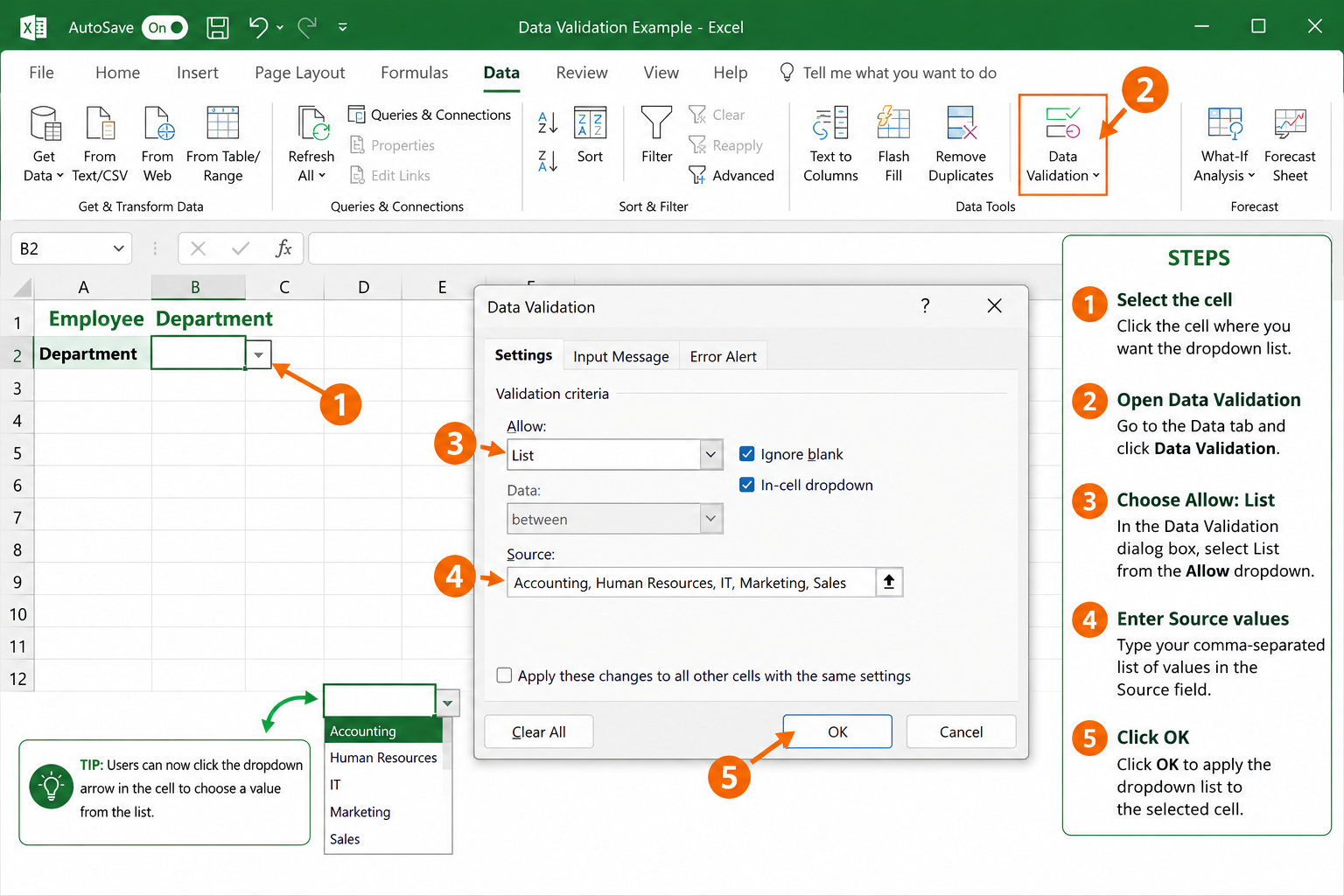
Step-by-step:
- Select the cell (or range of cells) where you want the dropdown to appear.
- Click the Data tab in the ribbon.
- Click Data Validation (in the Data Tools group). A dialog box opens.
- Under the Settings tab, open the Allow dropdown and choose List.
- In the Source field, either:
- Type your options separated by commas:
Yes,No,Maybe - Or click the range selector and highlight cells that contain your list items (e.g.,
$A$1:$A$5)
- Type your options separated by commas:
- Make sure In-cell dropdown is checked.
- Click OK.
That’s it. A small arrow now appears in the cell when it’s selected. [9]
Common mistake: Leaving a space after the comma in your source list (e.g.,
Yes, No) — Excel treats that space as part of the option, so the list item becomes ” No” with a leading space. Skip the spaces.
For a deeper walkthrough with screenshots, check out this dedicated guide on how to create a drop down list in Excel.
How to Add Data Validation Dropdown in Excel (and What the Options Mean)
Data Validation is the engine behind every Excel dropdown list. The dropdown list is a data validation rule — specifically, the “List” type. [2]
Inside the Data Validation dialog, there are three useful tabs:
| Tab | What It Does |
|---|---|
| Settings | Defines the list source and whether blanks are allowed |
| Input Message | Shows a tooltip when the cell is selected (optional but helpful) |
| Error Alert | Controls what happens if someone types an invalid entry |
Error Alert options:
- Stop — Rejects the entry entirely and forces a valid choice.
- Warning — Lets the user override and type their own value after a prompt.
- Information — Just notifies the user; accepts any entry.
Choose “Stop” when data integrity is critical (like a status field in a project tracker). Choose “Warning” or “Information” when you want to suggest options but allow flexibility. [6]
Can I Use a Dropdown List in Excel Without Data Validation?
Technically, yes — but it’s limited. Excel has a built-in shortcut called Pick From Drop-Down List (right-click a cell to find it, or press Alt + Down Arrow). This shows all unique values already typed in the column above the active cell as a quick-pick list.
The catch: It only works within a continuous column of existing data. You can’t define custom options, and it doesn’t enforce any rules. It’s handy for quick data entry but not a real substitute for Data Validation dropdowns. [4]
For anything beyond casual use, the Data Validation method is the right approach.
How to Make a Dropdown List from Another Sheet in Excel
You can absolutely pull your list options from a different sheet — and it’s actually a best practice for keeping your data organized. [3]
Method 1: Direct sheet reference
In the Source field of Data Validation, type a reference like:
=Sheet2!$A$1:$A$10
Method 2: Named Range (recommended)
- Go to the sheet with your list items.
- Select the range and go to Formulas → Define Name.
- Give it a name like
StatusOptions. - Back in Data Validation, type
=StatusOptionsin the Source field.
Named ranges are easier to maintain and read. If your list grows, just update the named range — the dropdown updates automatically. [7]
Edge case: If you share the workbook or protect sheets, named ranges are more reliable than direct sheet references, which can break if sheet names change.
What’s the Difference Between Dropdown and Data Validation in Excel?
These terms are often used interchangeably, but they’re not exactly the same thing. Data Validation is a broader Excel feature that can restrict cells to whole numbers, dates, text length, custom formulas, and more. A dropdown list is just one type of data validation rule — the “List” type. [2]
So every dropdown list in Excel is a data validation rule, but not every data validation rule creates a dropdown list.
How to Edit or Delete a Dropdown List in Excel
To edit a dropdown list:
- Select the cell with the dropdown.
- Go to Data → Data Validation.
- Update the Source field (add, remove, or change items).
- Click OK.
If the list source is a cell range, just edit the values in those cells directly — the dropdown updates automatically. [3]
To delete a dropdown list:
- Select the cell(s).
- Go to Data → Data Validation.
- Click Clear All at the bottom of the dialog, then OK.
This removes the validation rule but keeps any value already in the cell.
How to Copy a Dropdown List to Multiple Cells in Excel
The fastest way is Paste Special. Here’s how:
- Copy the cell that already has the dropdown (Ctrl+C).
- Select the destination cells.
- Press Ctrl+Alt+V to open Paste Special.
- Choose Validation and click OK.
This pastes only the data validation rule — not the cell’s value or formatting. [4]
Alternatively, if you’re setting up a new sheet, just select the entire column or a large range before opening Data Validation and apply the rule to all of them at once.
Can You Make a Dropdown List Dependent on Another Dropdown in Excel?
Yes — this is called a dependent (or cascading) dropdown list, and it’s one of the most powerful dropdown techniques in Excel. [7]
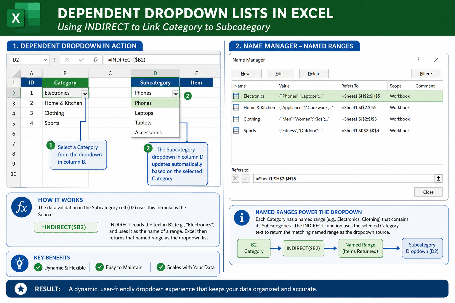
The basic approach:
- Create named ranges for each sub-list (e.g., a range named
Fruitscontaining Apple, Banana, Mango; a range namedVegetablescontaining Carrot, Broccoli, Spinach). - Create the first dropdown (Category) using Data Validation → List, with source
Fruits,Vegetables. - In the second dropdown cell, use Data Validation → List with source:
=INDIRECT(A2)(where A2 is the first dropdown cell).
When someone picks “Fruits” in the first dropdown, the second dropdown automatically shows only fruit options. [9]
Watch out: Named ranges must match the dropdown values exactly, including capitalization. “Fruits” and “fruits” are treated as different names.
How to Add a Dropdown List in Excel on Mac
Mac users follow the same core steps. The Data Validation dialog in Excel for Mac looks nearly identical to the Windows version. [2]
- Select your cell(s).
- Click the Data tab.
- Click Data Validation.
- Under Allow, choose List.
- Enter your source values or range.
- Click OK.
The main difference Mac users notice: keyboard shortcuts may vary slightly. For example, Alt+Down Arrow (Windows) becomes Option+Down Arrow on Mac to open a dropdown. Everything else works the same way.
If you’re newer to Excel on any platform, this beginner’s guide to using Excel is a good starting point.
What Happens If Someone Types Something Not on the Dropdown List?
It depends on how the Error Alert is configured in the Data Validation settings.
- Stop (default): Excel rejects the entry and shows an error message. The user must pick from the list or press Escape.
- Warning: Excel shows a message but lets the user click “Yes” to keep their typed value.
- Information: Excel shows a note but accepts the entry without any friction.
- No alert set: If the Error Alert tab is left unconfigured, Excel may accept the typed value silently (behavior can vary by version).
For strict data control — like a shared workbook used by a team — always set the alert to Stop and write a clear error message explaining what’s expected. [6]
How to Create a Dropdown List with a Formula in Excel
In Excel 365 and Excel 2021, you can use dynamic array formulas as a dropdown source. The most useful is UNIQUE, which automatically generates a deduplicated list from a data column.
Example:
- In a helper column, enter:
=UNIQUE(B2:B100)— this spills a unique list of values. - Select that spilled range (or use the spill reference like
=Sheet2!$D$2#) as your Data Validation source.
Now when new unique values appear in column B, the dropdown updates automatically — no manual editing needed. [7]
This approach works well for dashboards and reports where source data changes frequently. For more on Excel formulas, the complete beginner-to-pro guide for 2026 covers the essentials.
How to Make a Dropdown List Searchable in Excel
In Excel 365 (version 2306 and later), Microsoft added a built-in search box to dropdown lists. When you click a dropdown cell, a search field appears at the top of the list — just start typing and the list filters in real time. This feature rolls out automatically; no extra setup is needed. [2]
For older Excel versions, a common workaround is:
- Use a helper cell where the user types a partial search term.
- Use a FILTER formula to return matching items:
=FILTER(A2:A100, ISNUMBER(SEARCH(D1, A2:A100))). - Point the Data Validation source to that filtered spill range.
It’s more complex to set up but gives older Excel users a similar experience.
Why Isn’t My Dropdown List Working in Excel?
Here are the most common reasons a dropdown stops showing or behaving correctly:
| Problem | Likely Cause | Fix |
|---|---|---|
| Arrow doesn’t appear | “In-cell dropdown” checkbox is unchecked | Re-open Data Validation and check it |
| List is empty | Source range is on a different sheet but referenced incorrectly | Use a named range instead |
| Typed values are accepted despite Stop alert | Error Alert tab was never configured | Set Style to “Stop” in the Error Alert tab |
| Dependent dropdown shows wrong items | Named range doesn’t match the parent dropdown value exactly | Check capitalization and spacing in range names |
| Dropdown disappeared after copy/paste | Regular paste overwrites validation | Use Paste Special → Validation to preserve it |
If you’re working with protected sheets, also check that the cells with dropdowns are not locked before protection is applied — locked cells can’t be interacted with. See this guide on how to lock specific cells in Excel for how locking and protection interact.
FAQ
Q: How many items can a dropdown list have in Excel? A: There’s no hard limit on the number of items in a list range. However, if you type items directly in the Source field, the total character limit is 255 characters. Use a cell range for longer lists.
Q: Can I add color coding to dropdown list choices? A: Yes — use Conditional Formatting to apply different colors based on the selected value. For example, “Approved” turns green and “Rejected” turns red. See this guide on how to get a cell to change color based on its value.
Q: Does a dropdown list work in Excel Online? A: Yes. Excel Online (the browser version) supports Data Validation dropdowns for viewing and selecting. Creating or editing them in the browser has some limitations depending on your Microsoft 365 subscription tier.
Q: Can I add a dropdown list to a merged cell? A: Yes, but merged cells can cause issues with copying and pasting validation. It’s generally better to avoid merging cells in data entry areas. For more on merging, see how to merge cells in Excel using shortcut keys.
Q: How do I add a blank option to my dropdown list?
A: Simply include an empty entry in your source range (leave one cell blank), or add a comma at the start of a typed list: ,Yes,No,Maybe. The first item will be blank.
Q: Can I use a dropdown list in a table (Excel Table format)? A: Yes, and it works well. If the table column has a dropdown applied to one cell, Excel will often auto-fill the validation to new rows added to the table.
Q: Will a dropdown list slow down my Excel file? A: No. Dropdown lists via Data Validation are very lightweight and have no meaningful impact on file performance, even with hundreds of validated cells.
Q: Can I search within a dropdown list on older Excel versions? A: Not natively. The built-in search feature is only available in Excel 365 (recent builds). For older versions, a FILTER-formula workaround is the best option.
Conclusion
Adding a dropdown list in Excel is one of the most practical skills for anyone who works with spreadsheets regularly. The core method — Data → Data Validation → List — takes less than a minute once you know it, and it immediately improves the accuracy and consistency of your data.
Actionable next steps:
- Start simple: Add a dropdown to one column in a spreadsheet you use regularly (status fields, category columns, and yes/no fields are great candidates).
- Move your list to a separate sheet: Keep source data organized by putting list items on a dedicated “Lists” or “Reference” sheet, using named ranges for easy maintenance.
- Add color coding: Pair your dropdown with Conditional Formatting to make statuses visually obvious at a glance.
- Try dependent dropdowns: Once you’re comfortable, set up a two-level cascading dropdown using named ranges and the INDIRECT function.
- Protect your work: After setting up dropdowns, consider locking the validated cells so users can only interact with the dropdown — not accidentally delete the validation rule.
For a full video walkthrough and more Excel tips, explore the complete how-to guide on creating drop down lists in Excel.
References
[1] Watch – https://www.youtube.com/watch?v=-02SsHDW2lQ [2] Create A Drop Down List – https://support.microsoft.com/en-us/excel/get-started/create-a-drop-down-list [3] Add Or Remove Items From A Drop Down List – https://support.microsoft.com/en-us/office/add-or-remove-items-from-a-drop-down-list-0b26d3d1-3c4d-41f5-adb4-0addb82e8d2c [4] Drop Down List Excel – https://www.acuitytraining.co.uk/news-tips/drop-down-list-excel/ [6] Dropdown List Excel – https://techoutreach.extension.msstate.edu/sites/techoutreach.extension.msstate.edu/files/technology-tips/dropdown-list-excel.pdf [7] How To Create Drop Down List In Excel – https://www.geeksforgeeks.org/excel/how-to-create-drop-down-list-in-excel/ [9] Drop Down List – https://www.excel-easy.com/examples/drop-down-list.html [10] Add A List Box Or Combo Box To A Worksheet In Excel – https://support.microsoft.com/en-us/office/add-a-list-box-or-combo-box-to-a-worksheet-in-excel-579e1958-f7f6-41ae-ba0c-c83cc6e40878