
Last updated: June 22, 2026
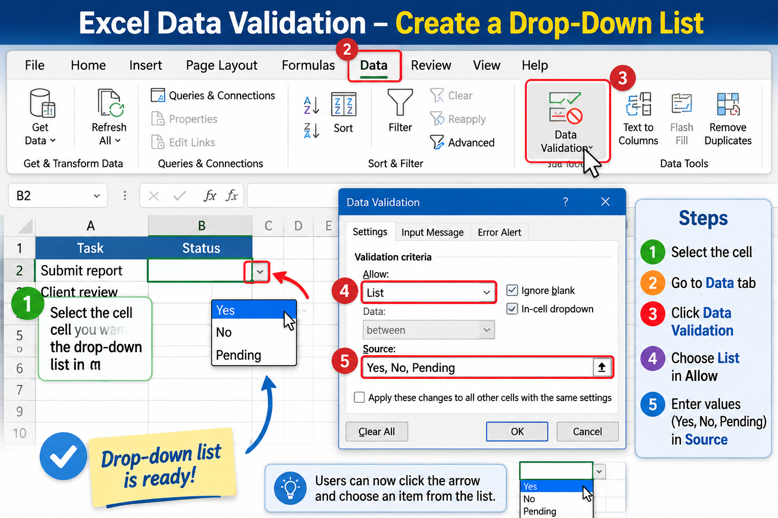
Quick Answer: To create a drop down list in Excel, select a cell, go to the Data tab, click Data Validation, choose List from the “Allow” menu, then type your items or point to a cell range. Click OK and the dropdown arrow appears immediately. The whole process takes under two minutes.
Key Takeaways
- Drop down lists in Excel are created through Data > Data Validation > List — no formulas required for basic use
- You can type items directly into the dialog box (comma-separated) or reference a cell range as the source
- Using an Excel Table as the source makes your list dynamic — it expands automatically when you add new items
- A named range keeps your source tidy and makes the validation formula easier to read
- You can copy a dropdown cell to apply the same validation to multiple cells at once
- Dropdown lists reduce data entry errors by limiting what users can type into a cell [6]
- You can add an input message and an error alert to guide users when they interact with the cell
- Cascading (dependent) dropdowns are possible using the INDIRECT function for more advanced setups
What Is a Drop Down List in Excel and Why Use One?
A drop down list in Excel is a data validation tool that restricts a cell to a predefined set of choices. When a user clicks the cell, a small arrow appears and a menu opens with the allowed options.
Why it matters:
- 🚫 Prevents typos and inconsistent entries (e.g., “Pending” vs “pending” vs “PENDING”)
- ✅ Speeds up data entry — one click instead of typing
- 📊 Makes filtering and reporting more reliable because values stay consistent
- 👥 Ideal for shared workbooks where multiple people enter data
Drop down lists are especially useful in forms, trackers, dashboards, and any spreadsheet where the same set of values repeats. If you’re just getting started with Excel, check out this beginner’s guide to using Excel step by step before diving into validation.
How to Create a Drop Down List in Excel: The Basic Method
The fastest way to create a drop down list in Excel is to type your options directly into the Data Validation dialog. This works best when you have a short, fixed list that won’t change often. [6]
Step-by-step:
- Select the cell (or range of cells) where you want the dropdown to appear
- Click the Data tab on the ribbon
- Click Data Validation in the Data Tools group
- In the dialog box, under the Settings tab, open the Allow dropdown and choose List
- In the Source field, type your items separated by commas — for example:
Yes,No,Pending - Make sure In-cell dropdown is checked
- Click OK
That’s it. Click the cell and you’ll see the dropdown arrow. [9]
💡 Quick tip: To apply the same dropdown to a whole column, select the entire column before opening Data Validation. Or, after creating it on one cell, copy the cell and paste it (using Paste Special > Validation) to other cells.
Common mistake: Leaving spaces around commas in the source field (e.g., Yes, No, Pending). Excel includes those spaces in the option text, so “No” and ” No” become different values. Skip the spaces.
How to Create a Drop Down List in Excel Using a Cell Range
Typing items directly works for small lists, but pointing to a cell range is cleaner and easier to update. This method is the most common approach for real-world spreadsheets. [6]
Steps:
- Type your list items in a column somewhere in your workbook — for example,
Sheet2!A1:A5 - Select the cell where you want the dropdown
- Go to Data > Data Validation > List
- In the Source field, click the small range selector icon and highlight your list items
- Click OK
Choose this method if:
- Your list has more than 5–6 items
- You want to update the list in one place and have all dropdowns reflect the change
- Multiple dropdowns across the sheet share the same options
Edge case: If your source list is on a different sheet, Excel requires you to use a named range instead of a direct cross-sheet reference in the Source field (in older Excel versions). Define a named range first via Formulas > Name Manager, then type =YourRangeName in the Source field.
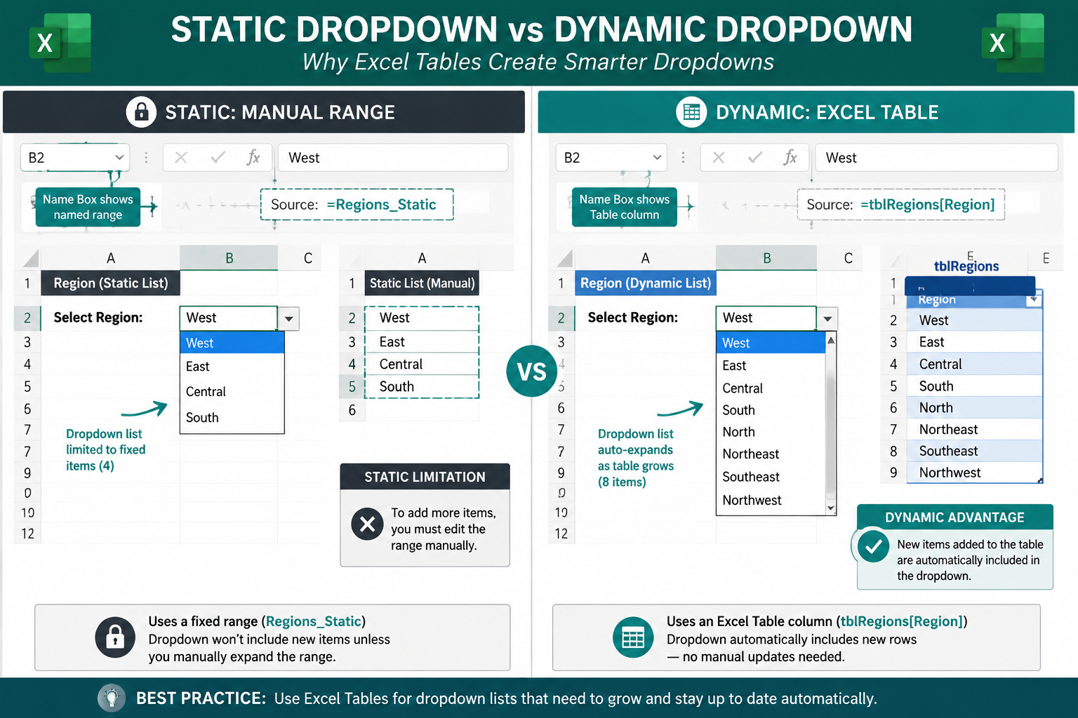
How to Make a Dynamic Drop Down List Using an Excel Table
A dynamic dropdown automatically includes new items when you add them to the source list. The cleanest way to achieve this is by formatting your source data as an Excel Table. [5]
How to set it up:
- Select your list items and press Ctrl + T to convert them to an Excel Table
- Give the table a meaningful name in the Table Design tab (e.g.,
StatusList) - Create a named range that references the table column: go to Formulas > Define Name, and in the “Refers to” field enter
=StatusList[Status](replace with your actual table and column names) - Use that named range as the Source in your Data Validation dialog
Now, whenever you add a new row to the table, the dropdown updates automatically — no need to edit the validation rule. This is a significant time-saver for growing lists. [5]
Why this beats a static range: A static range like $A$1:$A$10 won’t include an 11th item you add later. The table-based approach handles that for you.
Adding Input Messages and Error Alerts to Your Dropdown
Excel’s Data Validation dialog has two extra tabs that most people ignore: Input Message and Error Alert. Both are worth using in shared workbooks.
Input Message tab:
- Shows a small tooltip when the user selects the cell
- Use it to explain what the dropdown is for, e.g., “Select the current project status”
Error Alert tab:
- Controls what happens if someone types a value not in the list
- Stop (red X): Blocks the entry entirely — strictest option
- Warning (yellow !): Warns the user but allows them to override
- Information (blue i): Just shows a note, no restriction
For most data collection forms, Stop is the right choice. For lists where occasional custom entries are acceptable, Warning works better.
How to Edit or Remove a Drop Down List in Excel
Editing a dropdown is straightforward. Select any cell that has the dropdown, go back to Data > Data Validation, and change the source or items in the Settings tab. Click OK to save.
To remove a dropdown entirely:
- Select the cell(s) with the dropdown
- Go to Data > Data Validation
- Click Clear All at the bottom of the dialog
- Click OK
To find all cells with dropdowns in a sheet:
- Press Ctrl + G (Go To), click Special, then select Data Validation > All. Excel highlights every cell with a validation rule — handy for auditing a workbook someone else built.
If you want to protect your dropdown cells from being accidentally deleted or overwritten, pair this with cell locking in Excel to keep your validation rules intact.
Dependent (Cascading) Drop Down Lists
A dependent dropdown changes its options based on what the user selected in a previous dropdown. For example, selecting “Fruit” in column A shows only fruit names in column B’s dropdown.
The basic approach uses the INDIRECT function:
- Create named ranges for each sub-list (e.g., a range named
Fruitwith apple, banana, mango; a range namedVegetablewith carrot, spinach, onion) - In the first dropdown, list the category names (Fruit, Vegetable)
- In the second dropdown’s Source field, enter:
=INDIRECT(A2)— where A2 is the cell with the first dropdown
Important constraint: Named ranges used with INDIRECT must match the options in the first list exactly, including capitalization. “Fruit” and “fruit” won’t match.
This is one of the more advanced Excel techniques. For more Excel skills to build on, the how to learn MS Excel in 24 hours guide covers a solid learning path.
Common Mistakes When Creating Drop Down Lists in Excel
Even experienced users run into these issues:
| Mistake | What Happens | Fix |
|---|---|---|
| Spaces around commas in source | Options include leading/trailing spaces | Remove spaces: Yes,No not Yes, No |
| Source list on another sheet (no named range) | Validation dialog throws an error | Define a named range first |
| Static range doesn’t grow | New items don’t appear in dropdown | Use an Excel Table as source |
| Copying cell overwrites validation | Paste replaces the dropdown rule | Use Paste Special > Validation only |
| Forgetting to lock source cells | Users accidentally delete the list | Lock the source cells |
FAQ
Can you create a drop down list in Excel on a Mac? Yes. The steps are identical on Mac: Data tab > Data Validation > List. The dialog looks slightly different but all the same options are available.
Does a drop down list work in Excel Online (browser)? Yes, Excel for the web supports creating and using drop down lists via Data Validation. Some advanced features like dependent dropdowns may have minor limitations compared to the desktop app. [6]
How many items can a drop down list in Excel hold? There’s no hard item limit for range-based lists. For manually typed lists in the Source field, the total character limit is 255 characters including commas.
Can I search within a drop down list in Excel? Standard dropdown lists don’t have a built-in search. For long lists, consider using Excel’s AutoComplete feature or a more advanced combo box from the Developer tab.
How do I copy a drop down list to another cell? Copy the cell with the dropdown (Ctrl+C), then select the destination cell(s), right-click, choose Paste Special, and select Validation. This copies only the rule, not the cell content.
Can multiple cells share the same drop down list? Yes. Select all the cells you want to have the dropdown before opening Data Validation, and the rule applies to all of them at once.
What happens if I delete the source list cells? The dropdown stops working and shows an error. Always keep source list cells intact, or better yet, put them on a hidden sheet and lock them.
Can I add color coding to dropdown selections? Not directly through Data Validation, but you can use Conditional Formatting to color a cell based on which dropdown option is selected. Learn more about applying color based on cell value.
Conclusion
Creating a drop down list in Excel is one of the most practical data validation skills you can add to your toolkit. Start with the basic method — Data > Data Validation > List — and type a few comma-separated values to see it work immediately. Once that clicks, move to range-based lists for easier management, then graduate to Excel Table sources for fully dynamic dropdowns that maintain themselves.
Actionable next steps:
- Open any existing spreadsheet and add a simple Yes/No dropdown to a column you currently type manually
- Convert your source list to an Excel Table so it grows automatically
- Add an error alert to prevent invalid entries in shared workbooks
- Explore conditional formatting to visually highlight different dropdown selections
- Try the INDIRECT function for dependent dropdowns once you’re comfortable with the basics
For more Excel tips and techniques, browse the full Mark’s Excel Tips blog.
References
[5] Creating Dropdown List In Excel Sheet – https://www.samyoung.co.nz/2026/02/creating-dropdown-list-in-excel-sheet.html [6] Create A Drop Down List – https://support.microsoft.com/en-us/office/create-a-drop-down-list-7693307a-59ef-400a-b769-c5402dce407b [9] How Do I Create A Drop Down List – https://learn.microsoft.com/en-us/answers/questions/5449729/how-do-i-create-a-drop-down-list