Last updated: June 30, 2026
Quick Answer: To freeze a column in Excel, go to the View tab, click Freeze Panes, and select Freeze First Column. This locks column A so it stays visible while you scroll right. To freeze multiple columns, click the cell in the first row just to the right of the last column you want frozen, then choose Freeze Panes from the same menu. [2]
Key Takeaways
- Freezing a column keeps it visible on screen while you scroll horizontally through a large spreadsheet.
- The View > Freeze Panes menu handles all freeze options: first column, multiple columns, rows, or both at once.
- To freeze multiple columns, select the correct cell before clicking Freeze Panes — the freeze line appears to the left of the active cell.
- Mac users follow the same steps; the menu location is identical in Excel for Mac. [3]
- There is no direct keyboard shortcut to freeze panes, but you can access it via the Alt key sequence (Alt → W → F → C on Windows).
- Freezing does not affect your data — it only changes what you see on screen.
- Unfreezing is just as easy: View > Freeze Panes > Unfreeze Panes.
- Google Sheets and Excel Mobile both support column freezing with slightly different steps.
What Does Freezing a Column in Excel Do?
Freezing a column locks it in place visually so it stays on screen as you scroll right. The data itself does not move or change — only your view is affected.
This is especially useful for wide spreadsheets where the first column holds labels like customer names, product IDs, or dates. Without freezing, those labels scroll off screen and you lose track of which row you’re looking at. If you’re new to Excel navigation, the complete beginner-to-pro guide for 2026 covers this and many other essential skills.
What changes when you freeze:
- A thin vertical line appears between the frozen column(s) and the rest of the sheet.
- Scrolling right moves only the unfrozen columns — frozen ones stay put.
- The freeze applies only to your current view, not to anyone else’s unless they open the same saved file with freeze settings intact.
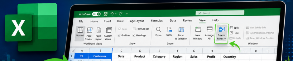
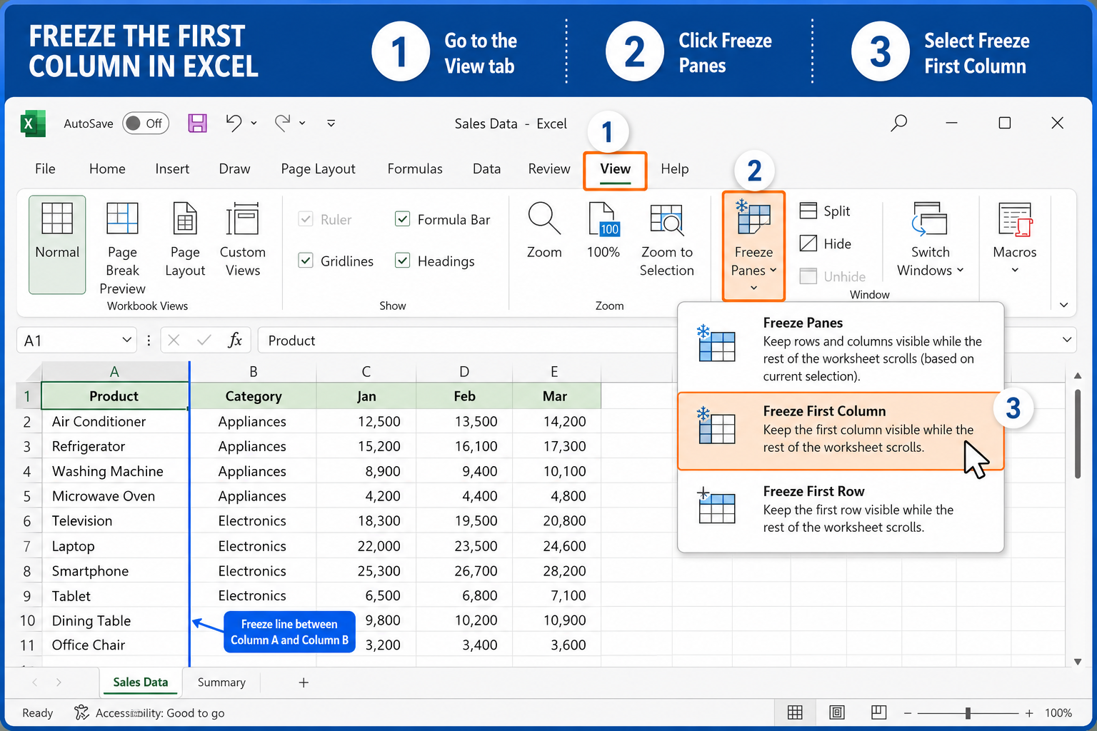
How to Freeze the First Column in Excel (Step by Step)
Freezing the first column is the most common use case and takes about three clicks. [2]
- Open your Excel workbook and navigate to the sheet you want to work on.
- Click the View tab in the ribbon at the top.
- Click Freeze Panes in the Window group.
- Select Freeze First Column from the dropdown.
A vertical line now appears between column A and column B. Scroll right — column A stays locked. That’s it.
💡 Quick tip: You don’t need to select any cell first when freezing just the first column. Excel handles it automatically.
For a detailed walkthrough on freeze panes alongside other Excel 365 navigation tricks, see how to freeze the top row and first column in Excel 365.
How to Freeze Multiple Columns in Excel
To freeze more than one column, you need to select a specific cell before applying the freeze — this is where most people go wrong.
The rule: Click the cell in row 1 of the first column you do not want frozen. The freeze line will appear to the left of that cell.
Example: To freeze columns A and B, click cell C1, then go to View > Freeze Panes > Freeze Panes (the top option, not “Freeze First Column”). [2]
| Columns to Freeze | Cell to Select First | Menu Option to Click |
|---|---|---|
| Column A only | Any cell | Freeze First Column |
| Columns A and B | C1 | Freeze Panes |
| Columns A, B, and C | D1 | Freeze Panes |
Common mistake: Selecting a cell in row 3 instead of row 1 will freeze both rows and columns simultaneously (which may or may not be what you want — see the section below on freezing both at once).
How to Freeze a Column and Row at the Same Time in Excel
Excel lets you lock both a row and a column simultaneously by selecting the intersection cell. Click the cell that is one row below the last row you want frozen and one column to the right of the last column you want frozen. [2]
Example: To freeze row 1 and column A at the same time, click cell B2, then go to View > Freeze Panes > Freeze Panes.
Both a horizontal and vertical freeze line will appear. Row 1 and column A stay visible no matter where you scroll.
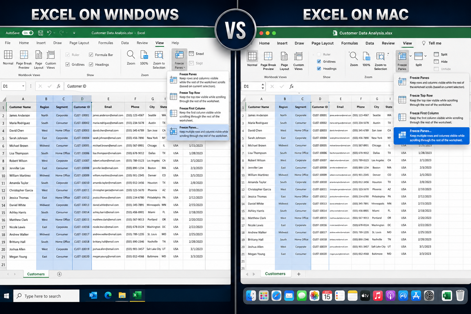
How to Freeze a Column in Excel on Mac
Mac users follow the exact same steps as Windows. The Freeze Panes option lives in the same place. [3]
- Open Excel on your Mac.
- Click the View tab in the ribbon.
- Click Freeze Panes.
- Choose Freeze First Column (or select a cell first for multiple columns).
The only difference: if you’re using an older Mac version of Excel that doesn’t show the full ribbon, go to Window > Freeze Panes from the top menu bar instead. [3]
How to Unfreeze a Column in Excel
Unfreezing is a single menu action. Go to View > Freeze Panes > Unfreeze Panes. The “Unfreeze Panes” option only appears when a freeze is already active — if you don’t see it, nothing is currently frozen.
There’s no need to select a specific cell before unfreezing. Excel removes all freeze panes at once; you can’t unfreeze just one column while keeping another frozen.
Is There a Keyboard Shortcut to Freeze Columns in Excel?
There’s no single dedicated keyboard shortcut, but you can use the Alt key sequence on Windows to get there without touching the mouse. [9]
Press these keys in sequence (not simultaneously):
- Alt → W → F → F — opens Freeze Panes (general)
- Alt → W → F → C — Freeze First Column
- Alt → W → F → R — Freeze Top Row
On Mac, there’s no equivalent keyboard shortcut for freeze panes natively, but you can assign a custom shortcut via System Preferences if needed.
For more Excel keyboard shortcuts, the Excel shortcuts cheat sheet is a handy reference.
Freeze Column in Excel Not Working — What to Do
If the freeze isn’t sticking or the option is grayed out, one of these issues is usually the cause. [7]
Check these first:
- The workbook is protected. Sheet protection disables freeze panes. Go to Review > Unprotect Sheet and try again.
- You’re in cell editing mode. Press Escape to exit editing mode before accessing the View menu.
- The file is in Compatibility Mode (.xls format). Save as .xlsx and try again.
- You already have a freeze active in an unexpected place. Unfreeze first (View > Freeze Panes > Unfreeze Panes), then reapply.
If the freeze line appears but columns still scroll, check that you didn’t accidentally place the freeze line after column A when you intended to freeze it.
What Happens When You Freeze a Column Then Add New Data?
Freezing does not interfere with adding, editing, or deleting data. New columns added to the right of the frozen section scroll normally. New columns inserted within the frozen section (for example, inserting a column between A and B when both are frozen) will also become frozen automatically because they fall within the frozen range. [4]
Edge case: If you insert a column to the left of your freeze line, the freeze line shifts one column to the right to compensate. This can sometimes cause confusion — just check the freeze line position after inserting columns near the frozen area.
Difference Between Freeze Panes and Split Screen in Excel
These two features look similar but behave differently. Freeze panes lock rows or columns so they stay visible while you scroll. Split screen divides the worksheet window into separate panes that can each scroll independently. [2]
| Feature | Freeze Panes | Split Screen |
|---|---|---|
| Purpose | Keep headers visible | View two parts of a sheet at once |
| Scrolling | Frozen area stays fixed | Each pane scrolls independently |
| Use case | Large datasets with headers | Comparing data in different areas |
| Found in | View > Freeze Panes | View > Split |
Choose Freeze Panes if you want column or row labels always visible. Choose Split if you want to compare two distant sections of the same sheet side by side.
How to Freeze Columns in Google Sheets Instead
Google Sheets handles column freezing through a different menu path, but the concept is identical.
- Open your Google Sheet.
- Click View in the top menu.
- Hover over Freeze.
- Select 1 column (or 2 columns, or Up to current column for more).
Alternatively, drag the thick gray bar at the top-left corner of the sheet (where row numbers and column letters meet) to the right to set the freeze point visually.
Google Sheets does not use the term “Freeze Panes” — it just says “Freeze.” The behavior is the same. If you’re working across both platforms, the how to use Excel for beginners step by step guide covers key differences between Excel and Sheets worth knowing.
Can You Freeze Columns in Excel on Mobile?
Yes, Excel on mobile (iOS and Android) supports freeze panes, though the interface is different. [4]
On Excel Mobile:
- Tap the cell to the right of the column(s) you want to freeze.
- Tap the View tab (you may need to scroll the ribbon).
- Tap Freeze Panes.
The freeze applies and a line appears on screen. Note that the mobile version has fewer options — you may not see separate “Freeze First Column” and “Freeze Top Row” shortcuts, just the general “Freeze Panes” option.
How to Freeze a Column in Older Versions of Excel (2010 and Earlier)
The steps for Excel 2010 are nearly identical to modern versions. The Freeze Panes button is in the same location: View tab > Window group > Freeze Panes. [9]
In Excel 2003 and earlier (pre-ribbon), the path is: Window menu > Freeze Panes. You still need to select the correct cell first to control which columns get frozen — the same intersection-cell rule applies.
One difference in older versions: there’s no separate “Freeze First Column” shortcut. You must click cell B1 first, then choose Freeze Panes from the Window menu.
FAQ
Q: Does freezing a column affect printing? A: No. Freeze panes only affect the on-screen view. To repeat columns on every printed page, use Page Layout > Print Titles instead.
Q: Can I freeze a column that isn’t column A? A: Not directly. Excel’s freeze panes always start from the leftmost column. You can’t freeze, say, column C without also freezing columns A and B.
Q: Will my freeze settings save when I close the file? A: Yes. Freeze pane settings are saved with the workbook. Anyone who opens the file will see the same freeze applied.
Q: Can I freeze more than one non-adjacent column? A: No. Excel only supports freezing a contiguous block of columns starting from column A.
Q: Why does my freeze line appear in the wrong place? A: You likely had the wrong cell selected before clicking Freeze Panes. Unfreeze first, select the correct cell (row 1, one column to the right of your last desired frozen column), then reapply.
Q: Does freezing columns slow down Excel? A: No. Freeze panes have no measurable impact on file performance.
Q: Can I freeze a column in Excel Online (browser version)? A: Yes. Excel Online supports freeze panes via View > Freeze Panes, with the same options as the desktop version.
Q: What’s the fastest way to freeze the first column? A: Use the keyboard sequence Alt → W → F → C on Windows. No mouse needed.
Conclusion
Knowing how to freeze a column in Excel is one of those small skills that saves real time every day. The core method — View > Freeze Panes > Freeze First Column — takes seconds to apply and works across Windows, Mac, Excel Online, and mobile. For multiple columns, the key is selecting the right cell in row 1 before applying the freeze.
Your next steps:
- Open a wide spreadsheet you work with regularly and freeze the first column right now.
- If you use row headers too, try freezing both a row and column at the same time using the intersection-cell method.
- Explore related navigation skills like expanding all columns with shortcut keys to keep your spreadsheets clean and easy to read.
- If you’re building complex sheets, pair freeze panes with conditional formatting traffic lights to make key data stand out at a glance.
Freeze panes won’t solve every spreadsheet problem, but for large datasets with headers, it’s one of the most practical tools Excel offers.
References
[2] Freeze Panes To Lock Rows And Columns – https://support.microsoft.com/en-us/office/freeze-panes-to-lock-rows-and-columns-dab2ffc9-020d-4026-8121-67dd25f2508f [3] Freeze Panes To Lock The First Row Or Column In Excel For Mac – https://support.microsoft.com/en-us/excel/freeze-panes-to-lock-the-first-row-or-column-in-excel-for-mac [4] How To Freeze Cells And Columns In Excel – https://www.asus.com/in/content/how-to-freeze-cells-and-columns-in-excel/ [7] Freeze Cells In Excel – https://www.wikihow.com/Freeze-Cells-in-Excel [9] Freeze Columns In Excel – https://www.indeed.com/career-advice/career-development/freeze-columns-in-excel