
Hello, and welcome to Mark’s Excel Tips. Today, we are going to show you how to freeze the top row, and first column at the same time in Excel 365. Let’s get started.
Click here to view our video tutorial.
Click here to download our PDF tutorial.
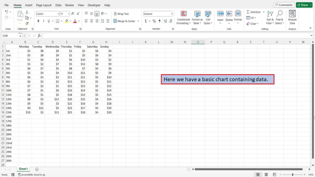
Here we have a basic chart containing data.
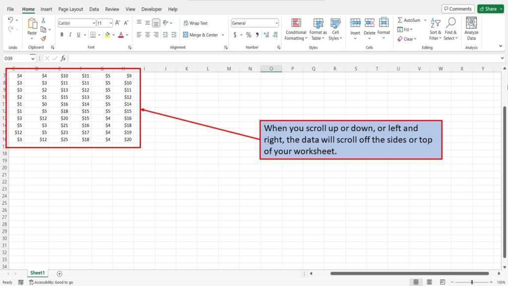
When you scroll up and down, or left and right, the data will scroll off the sides or top of your worksheet.
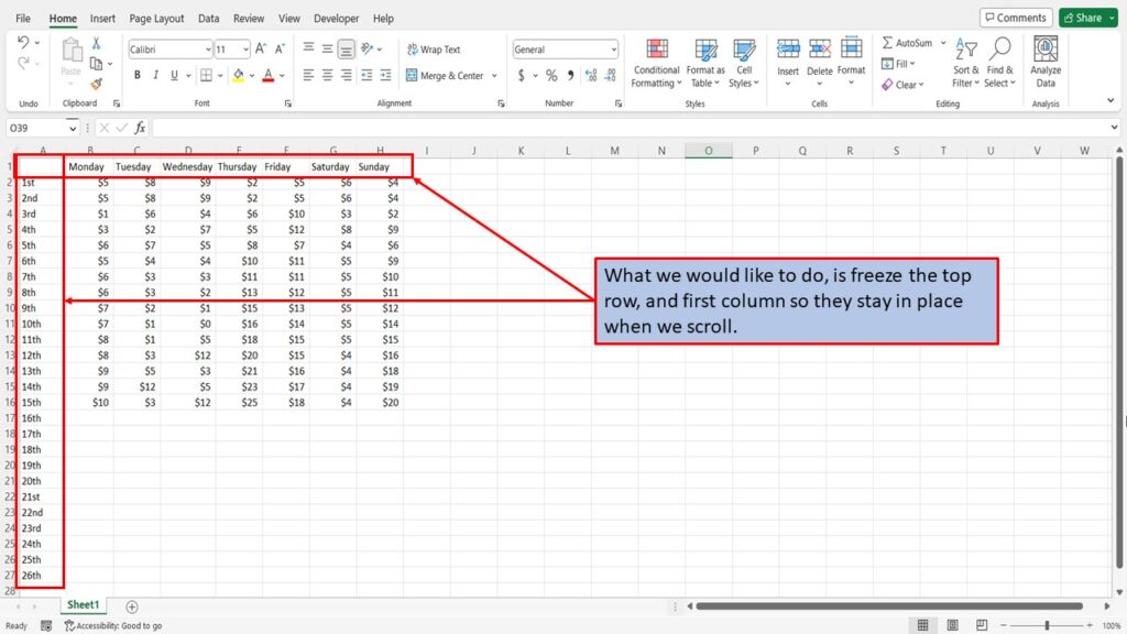
What we would like to do, is freeze the top row, and first column so they stay in place when we scroll.
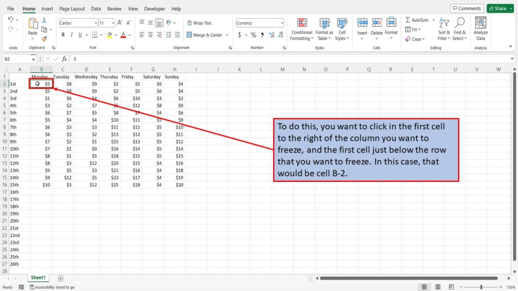
To do this, you want to click in the first cell to the right of the column you want to freeze, and the first cell just below the row that you want to freeze. In this case, that would be cell B-2.
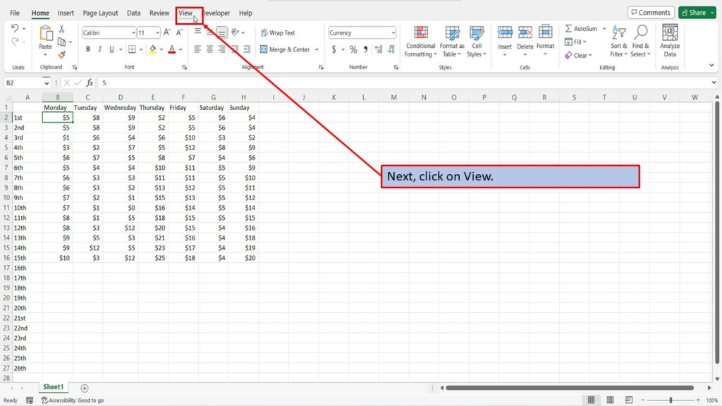
Next, click on View.
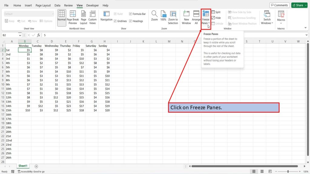
Click on Freeze Panes.
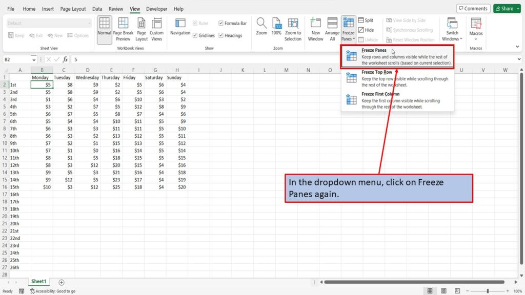
In the dropdown menu, click on Freeze Panes again.
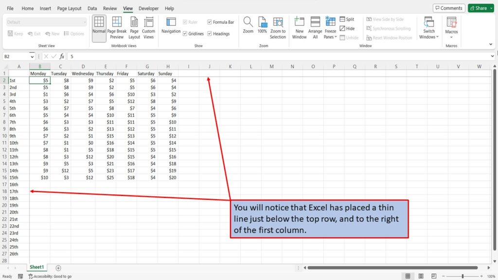
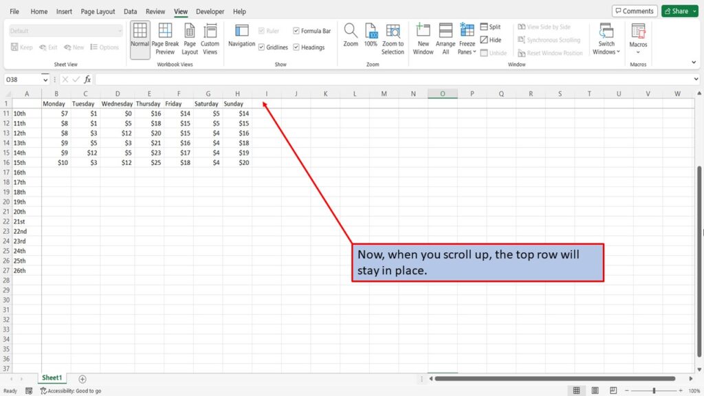
You will notice that Excel has placed a thin line just below the top row, and to the right of the first column.
Now, when you scroll up, the top row will stay in place.
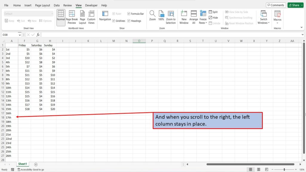
And when you scroll to the right, the left column stays in place.
View the Video Tutorial.
Download this tutorial in PDF by clicking the Download link below.