Master Spreadsheet Equations in Excel: Step-by-Step Examples for Real Workflows

Last updated: July 7, 2026

Quick Answer: To master spreadsheet equations in Excel, start with the core formula syntax (always begin with =), learn the ten most-used functions for business tasks, and practice applying them to real workflows like budgeting, inventory, and reporting. Most errors come from a handful of fixable mistakes, wrong cell references, missing dollar signs, and mismatched parentheses, all of which are easy to correct once you know what to look for.

Key Takeaways

Every Excel equation starts with = followed by a function name or math operator.
The ten most-used business formulas are SUM, AVERAGE, IF, VLOOKUP, INDEX/MATCH, COUNTIF, SUMIF, TEXT, IFERROR, and CONCATENATE.
Absolute references ($A$1) lock a cell; relative references (A1) shift when copied, knowing the difference prevents major calculation errors.
INDEX/MATCH is more flexible than VLOOKUP and handles left-side lookups that VLOOKUP cannot.
Nested IF statements work well for up to three conditions; beyond that, use IFS or a lookup table instead.
Common formula errors like #REF! and #VALUE! each have a specific cause and a quick fix.
Array formulas (including modern dynamic arrays like FILTER and UNIQUE) replace many multi-step manual processes.
Pivot tables beat formulas when you need to summarize large datasets quickly without writing any code.
Microsoft Copilot in Excel (2026) can suggest and build formulas automatically, speeding up complex workflows. [1]

What Formulas Should You Learn First If You’re New to Excel

Start with SUM, AVERAGE, IF, and COUNTA. These four cover the vast majority of everyday calculation tasks, adding numbers, finding a midpoint, making a simple yes/no decision, and counting filled cells. Once those feel natural, layer in VLOOKUP or INDEX/MATCH for lookups, and SUMIF/COUNTIF for conditional totals.

If you’re brand new to the application itself, the how to use Excel for beginners step by step guide covers the interface basics before you write a single formula.

Beginner priority order:

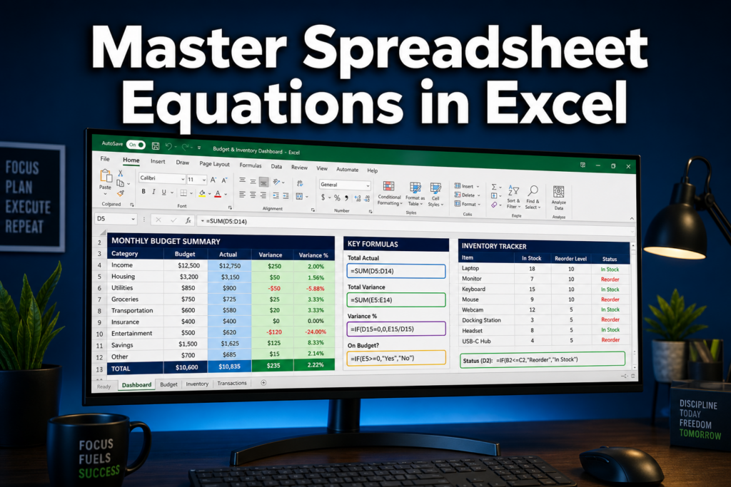
=SUM(A1:A10), adds a range [7]
=AVERAGE(A1:A10), finds the mean
=IF(A1>100,"Yes","No"), logical test
=COUNTA(A1:A10), counts non-empty cells
=VLOOKUP(value, table, col, FALSE), looks up a value in a table

💡 Quick tip: Press Alt + = to auto-insert a SUM formula instantly. See the Excel AutoSum shortcut guide for details.

How to Write a Formula in Excel for Beginners

Every Excel formula starts with an equals sign (=). Without it, Excel treats the entry as plain text. After the =, type a function name, then open parentheses, add your arguments (cell references, numbers, or text in quotes), and close the parentheses.

Step-by-step example, adding a column of sales:

Click the cell where you want the result (e.g., B11).
Type =SUM(
Click and drag to select B1:B10.
Type ) and press Enter.

Excel’s Formula AutoComplete shows a dropdown of matching functions as you type, reducing errors and speeding up entry. [2] The formula bar at the top always shows the full equation for the selected cell, so you can edit it any time.

Common beginner mistakes to avoid:

Forgetting the = sign
Typing text arguments without quotation marks (e.g., "Yes" not Yes)
Selecting the wrong range by one row

What Are the Most Common Excel Formulas Used in Business

The ten formulas below appear in almost every business spreadsheet, from small team trackers to enterprise financial models. Each one solves a specific real-world task.

Formula	What It Does	Real Workflow Example
SUM	Adds numbers	Monthly expense totals
AVERAGE	Calculates mean	Average sales per rep
IF	Logical test	Flag overdue invoices
VLOOKUP / INDEX-MATCH	Looks up values	Pull product prices from a catalog
SUMIF / COUNTIF	Conditional totals/counts	Total sales by region
IFERROR	Hides errors	Clean lookup results
TEXT	Formats numbers as text	Display dates in reports
CONCATENATE / &	Joins text	Combine first and last names

Microsoft maintains a full alphabetical function reference for every available formula. [6]

What’s the Difference Between Absolute and Relative Cell References

Relative references (like A1) shift automatically when a formula is copied to another cell. Absolute references (like $A$1) stay fixed no matter where you copy the formula. This distinction is one of the most important concepts for anyone working to master spreadsheet equations in Excel.

Example, tax rate calculation:

Say the tax rate is in cell D1. If the formula in B2 is =A2*D1 and you copy it down to B3, it becomes =A3*D2, wrong. Use =A2*$D$1 instead, and copying down gives =A3*$D$1, correct.

Reference types at a glance:

A1, both row and column shift (fully relative)
$A1, column locked, row shifts
A$1, row locked, column shifts
$A$1, fully locked (absolute)

Press F4 while clicking a cell reference in the formula bar to cycle through all four options quickly.

Best Excel Formulas for Financial Analysis and Budgeting

For budgeting and financial analysis, the most useful formulas are SUMIF, SUMIFS, PMT, NPV, and IF combined with comparison operators. These turn a plain data table into a working financial model.

Real budgeting workflow example:

Suppose column A has expense categories, column B has amounts, and you want the total for “Marketing”:

<code>=SUMIF(A:A,"Marketing",B:B)
</code>

For a loan payment calculation:

<code>=PMT(interest_rate/12, loan_term_months, -loan_amount)
</code>

For a ready-to-use starting point, the college budget template for Excel 365 shows these formulas already wired up in a real spreadsheet.

Key financial formulas:

PMT, monthly loan or mortgage payment
NPV, net present value of cash flows
IRR, internal rate of return
SUMIFS, totals filtered by multiple conditions
NETWORKDAYS.INTL, working days between two dates, with custom weekends [3]

How to Create Nested IF Statements in Excel

A nested IF places one IF formula inside another to test multiple conditions in sequence. Use this when a single true/false test isn’t enough, for example, assigning letter grades or tiered commission rates. [8]

Example, grade assignment:

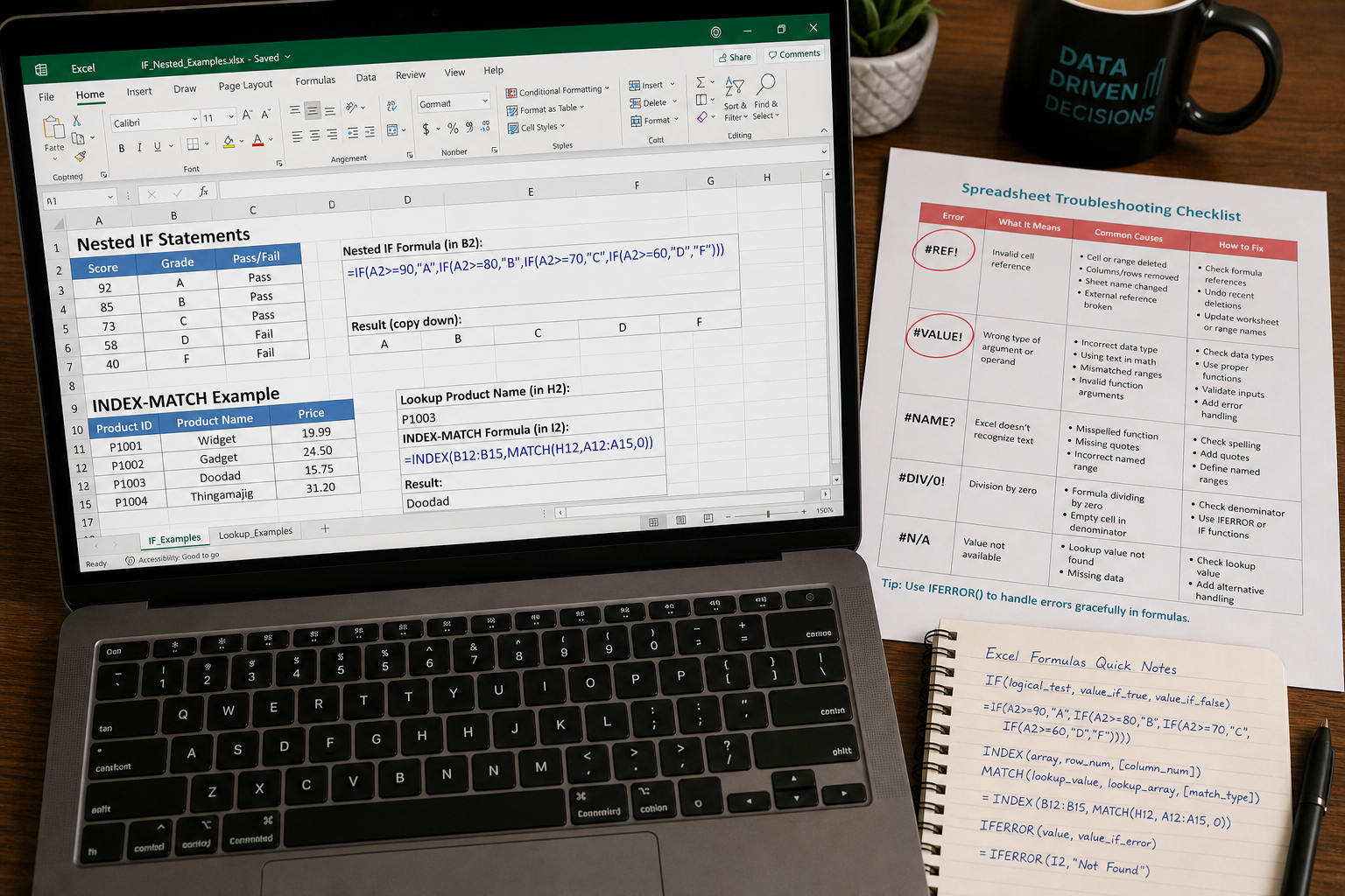
<code>=IF(A2>=90,"A",IF(A2>=80,"B",IF(A2>=70,"C","F")))
</code>

This checks the score in A2 against three thresholds in order. Excel evaluates left to right, so the first true condition wins.

When to use nested IF vs. alternatives:

1-3 conditions: Nested IF works fine.
4+ conditions: Use IFS(condition1, result1, condition2, result2, ...), cleaner and easier to read.
Category lookups: A VLOOKUP against a small reference table is often faster to maintain than a long nested IF.

⚠️ Excel allows up to 64 levels of nesting, but anything beyond 3-4 levels becomes very hard to debug. [2]

Can I Use VLOOKUP Instead of INDEX-MATCH, and When

VLOOKUP works well for simple right-side lookups, but INDEX/MATCH is more flexible and handles situations VLOOKUP cannot. For most new formulas written in 2026, INDEX/MATCH (or the newer XLOOKUP) is the better default choice.

VLOOKUP limitations:

Can only look up values to the right of the lookup column.
Breaks if columns are inserted or deleted (column number shifts).
Slightly slower on very large datasets.

Choose VLOOKUP if: The data is simple, the lookup column is always leftmost, and the file is shared with users on older Excel versions.

Choose INDEX/MATCH if: You need to look left, the column order might change, or you want a more resilient formula.

INDEX/MATCH example, pulling a price from column A using a product name in column C:

<code>=INDEX(A:A,MATCH(E2,C:C,0))
</code>

XLOOKUP (available in Excel 365 and Excel 2021+) simplifies this further:

<code>=XLOOKUP(E2,C:C,A:A)
</code>

How to Fix Formula Errors in Excel Like #REF! and #VALUE!

Each Excel error code points to a specific problem, and most are fixed in under a minute once you know the cause. Excel’s improved error detection tools now show explanations directly in the error tooltip. [4]

Common errors and fixes:

Error	Cause	Fix
`#REF!`	A referenced cell was deleted	Rewrite the formula pointing to valid cells
`#VALUE!`	Wrong data type (e.g., text in a math formula)	Check that all referenced cells contain numbers
`#DIV/0!`	Dividing by zero or an empty cell	Wrap with `IFERROR` or add an IF check
`#NAME?`	Function name misspelled	Check spelling; use Formula AutoComplete
`#N/A`	Lookup value not found	Use `IFERROR` or `IFNA` to show a custom message
`#NUM!`	Invalid numeric value	Check for negative numbers in square root or log functions

Wrap any error-prone formula with IFERROR:

<code>=IFERROR(VLOOKUP(A2,Sheet2!A:B,2,0),"Not found")
</code>

How to Combine Multiple Formulas in One Cell

Combining formulas means nesting one function inside another as an argument. This is how you build equations that do real work, for example, calculating a conditional average or formatting a lookup result. [2]

Example, show “High” or “Low” based on whether a value is above the column average:

<code>=IF(B2>AVERAGE(B:B),"High","Low")
</code>

Example, clean up a VLOOKUP result and format it as currency text:

<code>=TEXT(IFERROR(VLOOKUP(A2,PriceTable,2,0),0),"$#,##0.00")
</code>

Tips for combining formulas cleanly:

Build from the inside out, write the inner formula first and confirm it works, then wrap it.
Use the Evaluate Formula tool (Formulas tab → Evaluate Formula) to step through each layer.
Add line breaks in the formula bar (Alt + Enter) to make long formulas more readable.

Excel Formulas for Data Analysis and Reporting Workflows

For data analysis and reporting, the most productive formulas are SUMIFS, COUNTIFS, AVERAGEIFS, TEXT, and the dynamic array functions FILTER, SORT, and UNIQUE. These let you build self-updating reports without manually re-sorting or re-filtering data.

To master spreadsheet equations in Excel for reporting workflows, pair these formulas with structured Excel Tables (Insert → Table). Tables auto-expand when new rows are added, so formulas referencing them stay accurate without manual updates.

Reporting workflow example, weekly sales summary:

<code>=SUMIFS(Sales[Amount], Sales[Region], "North", Sales[Week], G2)
</code>

This totals sales for the North region in the week shown in G2, fully dynamic as the source data grows.

For visual reporting, pairing these formulas with charts makes trends immediately visible. The Excel chart tips series covers how to connect tables to charts so visuals update automatically.

How Do Array Formulas Work in Modern Excel

Array formulas calculate across multiple values at once and return either a single result or a range of results (called a “spill”). In modern Excel 365, dynamic array functions like FILTER, SORT, UNIQUE, and SEQUENCE work automatically without needing Ctrl+Shift+Enter. [3]

Example, list all sales over $500 from a dataset:

<code>=FILTER(A2:B50, B2:B50>500)
</code>

This spills a filtered list starting from the cell where you enter it, no helper columns needed.

Legacy array formulas (entered with Ctrl+Shift+Enter in older Excel versions) still work but are largely replaced by these newer dynamic functions in Excel 365.

When array formulas shine:

Extracting unique values from a list (UNIQUE)
Generating a numbered sequence automatically (SEQUENCE)
Filtering data without using the Filter button (FILTER)
Applying a custom calculation across every row or column (BYROW, BYCOL) [5]

When Should I Use Pivot Tables Instead of Formulas

Use a pivot table when you need to summarize, group, or cross-tabulate a large dataset quickly and the structure of the summary might change. Use formulas when you need a calculation embedded in a specific cell that feeds other formulas or updates automatically based on live inputs.

Choose a Pivot Table if:

You want to drag and drop to change the summary view.
You’re exploring data and don’t know exactly what groupings you need yet.
The dataset has hundreds or thousands of rows.

Choose Formulas if:

The output feeds into another calculation.
You need the result to update live as source data changes.
The layout must stay fixed (e.g., a printed report template).

For chart-based summaries from unsummarized data, Pivot Charts combine both approaches in one step.

Excel Formulas vs. Google Sheets: Which Is Better

Excel has a larger function library, better performance on large datasets, and more advanced features like Power Query and Copilot AI. Google Sheets wins on real-time collaboration and zero cost. For professional financial modeling or complex data workflows, Excel is still the stronger tool in 2026.

Key differences:

Unique to Excel: Power Query, Power Pivot, XLOOKUP (older Sheets versions), Copilot AI formula suggestions [1], BYCOL/BYROW [5]
Unique to Google Sheets: IMPORTRANGE (pull data from another sheet file), GOOGLEFINANCE (live stock prices), free with a Google account
Both support: FILTER, SORT, UNIQUE, IF, SUMIFS, VLOOKUP, and most common functions

Choose Excel if you work with large files, need advanced financial functions, or your organization uses Microsoft 365.
Choose Google Sheets if your team collaborates in real time across devices and cost is a priority.

Common Mistakes People Make With Excel Formulas

The most common formula mistakes are using relative references when absolute ones are needed, hardcoding values that should be cell references, and building formulas too complex to troubleshoot. Each of these is avoidable with a small habit change.

Top mistakes and how to fix them:

Forgetting $ signs, causes formulas to shift incorrectly when copied. Fix: press F4 to toggle absolute references.
Hardcoding numbers, e.g., =A1*0.08 instead of =A1*$B$1 (where B1 holds the rate). Fix: always reference a cell for values that might change.
Circular references, a formula that refers back to its own cell. Fix: check Formulas → Error Checking → Circular References.
Mixing data types, text stored as numbers (or vice versa) breaks SUM and AVERAGE. Fix: use VALUE() to convert, or check cell formatting.
Not using IFERROR, raw #N/A or #DIV/0! errors in a report look unprofessional and break downstream formulas.
Over-nesting, building a 6-level nested IF that nobody can read six months later. Fix: use IFS or a lookup table.

For more hands-on practice with Excel fundamentals, the how to use Excel for data entry guide covers clean data habits that prevent many of these errors before they start.

FAQ

Q: What’s the fastest way to sum a column in Excel?
Click the cell below the column, then press Alt + =. Excel inserts a SUM formula automatically and selects the range above.

Q: How do I make a formula not change when I copy it?
Add $ signs to lock the reference: $A$1 stays fixed in any direction. Press F4 while the cursor is on a cell reference in the formula bar to add dollar signs automatically.

Q: What does #REF! mean in Excel?
#REF! means the formula is pointing to a cell that no longer exists, usually because a row or column was deleted. Rewrite the formula to reference valid cells.

Q: Is XLOOKUP better than VLOOKUP?
Yes, for most use cases. XLOOKUP can look in any direction, doesn’t require a column number, and returns a custom value when nothing is found. It’s available in Excel 365 and Excel 2021+.

Q: How many IF statements can I nest in one formula?
Excel supports up to 64 nested IF levels, but anything beyond 3-4 becomes very hard to read and debug. Use the IFS function for cleaner multi-condition logic.

Q: What is a dynamic array formula?
A dynamic array formula returns multiple results that “spill” into neighboring cells automatically. Functions like FILTER, SORT, and UNIQUE work this way in Excel 365 without any special entry method.

Q: Can Excel write formulas for me?
Yes. Microsoft Copilot in Excel (available with a Microsoft 365 subscription) can generate and explain formulas based on a plain-language description of what you want to calculate. [1]

Q: How do I find which formula is causing an error?
Go to Formulas → Error Checking, or use Formulas → Evaluate Formula to step through each part of a complex equation one layer at a time.

Q: When should I use SUMIF vs. SUMIFS?
Use SUMIF for one condition. Use SUMIFS when you need two or more conditions, for example, total sales for a specific region AND a specific month.

Q: Do Excel keyboard shortcuts work with formulas?
Absolutely. Shortcuts like F2 (edit a cell), F4 (toggle reference type), and Ctrl+` (show all formulas) save significant time. The 50 time-saving Excel keyboard shortcuts guide covers the most useful ones.

Conclusion

The path to mastering spreadsheet equations in Excel runs through real tasks, not abstract memorization. Start with SUM, IF, and a basic lookup formula. Apply them to an actual budget, an inventory list, or a grading sheet. Fix the first #REF! error you encounter, understand why it happened, and you’ll never make that mistake again.

Actionable next steps:

This week: Build a simple budget using SUM, AVERAGE, and SUMIF on real numbers from your own life or work.
Next week: Replace one VLOOKUP with INDEX/MATCH or XLOOKUP and compare the results.
This month: Learn one dynamic array function (start with FILTER or UNIQUE) and apply it to a reporting task.
Ongoing: Use the Excel How To Videos library for visual walkthroughs as new formula questions come up.

Every complex Excel model started with someone typing =SUM( for the first time. The formulas covered here, applied consistently to real workflows, are enough to handle the vast majority of business spreadsheet tasks you’ll ever encounter.

References

[1] Excel – https://support.microsoft.com/en-us/excel?utm_source=openai
[2] Using Functions And Nested Functions In Excel Formulas – https://support.microsoft.com/en-US/Excel/using-functions-and-nested-functions-in-excel-formulas?utm_source=openai
[3] What S New Changes Made To Excel Functions – https://support.microsoft.com/en-us/excel/what-s-new-changes-made-to-excel-functions?utm_source=openai
[4] Detect Formula Errors In Excel – https://support.microsoft.com/en-us/Excel/detect-formula-errors-in-excel?utm_source=openai
[5] Logical Functions Reference – https://support.microsoft.com/en-us/excel/logical-functions-reference?utm_source=openai
[6] Excel Functions Alphabetical – https://support.microsoft.com/en-us/excel/excel-functions-alphabetical?utm_source=openai
[7] Excel Easy – SUM Examples – https://www.excel-easy.com/examples/sum.html?utm_source=openai
[8] Create Conditional Formulas – https://support.microsoft.com/en-US/Excel/create-conditional-formulas?utm_source=openai