How to Write Spreadsheet Formulas: A Beginner-to-Advanced Guide

Last updated: July 6, 2026

Quick Answer: Every spreadsheet formula starts with an equals sign (=), followed by functions, cell references, operators, and values. To write one, click a cell, type =, then build your expression using function names like SUM or IF, cell addresses like A1, and operators like + or *. Press Enter and the spreadsheet calculates the result instantly.

Key Takeaways

All formulas must begin with =, without it, the spreadsheet treats your entry as plain text [1]
Cell references (like B2 or D5) let formulas update automatically when data changes
Absolute references ($B$2) stay fixed; relative references (B2) shift when you copy a formula
SUM, IF, VLOOKUP, and AVERAGE cover the majority of everyday spreadsheet tasks [4]
Nesting means placing one formula inside another, powerful, but keep it readable
Google Sheets and Excel share most core formulas; differences are minor for beginners
You do not need to memorize every formula, the built-in function library and autocomplete handle that
Common errors like #REF!, #VALUE!, and #DIV/0! each have a specific, fixable cause
Array formulas let one formula process an entire range at once, Excel 365 makes this automatic
The fastest way to apply a formula to hundreds of rows is to double-click the fill handle

What Are the Basic Spreadsheet Formula Rules You Need to Know?

Every formula in Excel or Google Sheets follows the same core rules, regardless of complexity. Master these and the rest falls into place. [1]

The non-negotiables:

Start with =, this signals to the spreadsheet that a calculation is coming, not text [1]
Use cell references instead of typed numbers wherever possible (e.g., =A1+B1 rather than =5+3) so results update when data changes
Follow standard math order, multiplication and division happen before addition and subtraction; use parentheses to control the order [2]
Formulas can be up to 8,192 characters long in Excel, so there’s plenty of room for complex logic [2]
Function names are not case-sensitive, =sum(a1:a10) works the same as =SUM(A1:A10)

Operators you’ll use constantly:

Operator	Meaning	Example
`+`	Add	`=A1+B1`
`-`	Subtract	`=A1-B1`
`*`	Multiply	`=A1*B1`
`/`	Divide	`=A1/B1`
`^`	Exponent	`=A1^2`
`&`	Join text	`=A1&" "&B1`
`>`, `<`, `=`	Compare	`=A1>100`

If you’re brand new to Excel, the how to use Excel for beginners step by step guide is a great place to start before diving into formulas.

How Do I Write a Simple Formula to Add Numbers in Excel?

To add numbers in Excel, click an empty cell, type =SUM(, select the range you want to add, close the parenthesis, and press Enter. For example, =SUM(A1:A10) adds every number from A1 through A10. [2]

Three ways to add numbers:

Manual addition: =A1+A2+A3, fine for two or three cells, tedious for more
SUM function: =SUM(A1:A10), the standard approach for any range
AutoSum shortcut: Select the cell below your column of numbers and press Alt + =, Excel writes the SUM formula for you

💡 Quick tip: The colon (:) means “through”, so A1:A10 means cells A1 through A10. A comma means individual cells: =SUM(A1,A5,A9) adds just those three.

For a deeper look at adding rows, check out how to add up a row of numbers in Excel.

How Do I Write a Simple Formula to Add Numbers in Excel?

What’s the Difference Between Absolute and Relative Cell References?

A relative reference (like B2) shifts automatically when you copy a formula to another cell. An absolute reference (like $B$2) stays locked on that exact cell no matter where you copy the formula. This distinction is one of the most important concepts in spreadsheet formula writing. [1]

When to use each:

Relative (B2): Use when each row or column should reference its own corresponding cell. Example: =B2*C2 copied down a column will become =B3*C3, =B4*C4, and so on automatically.
Absolute ($B$2): Use when all rows should reference the same cell, like a tax rate stored in one place. Example: =B2*$D$1 keeps $D$1 fixed while B2 shifts.
Mixed ($B2 or B$2): Locks either the column or the row, but not both. Useful in multiplication tables.

Shortcut: Press F4 after clicking a cell reference in the formula bar to cycle through all four reference types.

Common mistake: Forgetting to use $ when copying a formula that references a fixed value (like a percentage or rate). The formula copies fine but produces wrong results because the reference drifts.

How Do I Use IF Statements in Spreadsheet Formulas?

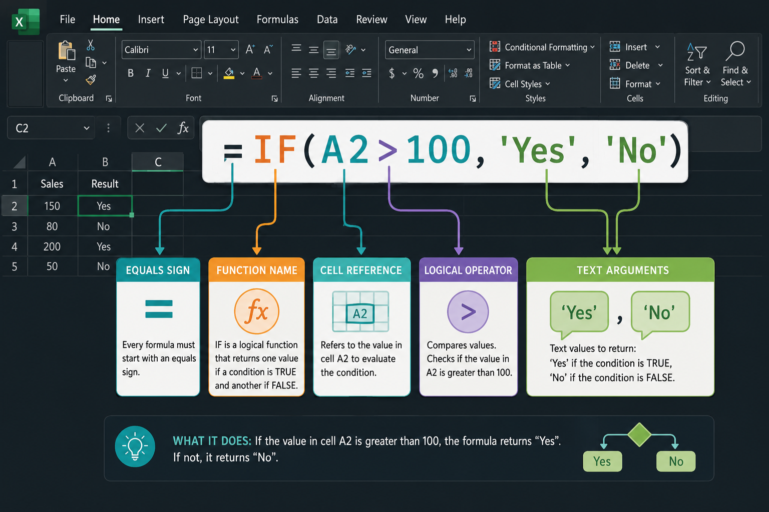
IF checks whether a condition is true or false and returns one result for true, another for false. The syntax is: =IF(condition, value_if_true, value_if_false). [4]

Example: =IF(B2>=60, "Pass", "Fail"), if the score in B2 is 60 or higher, it shows “Pass”; otherwise “Fail.”

Building more complex logic:

AND: =IF(AND(B2>=60, C2="Complete"), "Pass", "Fail"), both conditions must be true
OR: =IF(OR(B2>=60, C2="Exempt"), "Pass", "Fail"), either condition triggers true
Nested IF: =IF(B2>=90, "A", IF(B2>=80, "B", IF(B2>=70, "C", "F"))), chains multiple conditions

⚠️ Edge case: Nested IFs get hard to read beyond three levels. In Excel 365 and Google Sheets, IFS is cleaner: =IFS(B2>=90,"A", B2>=80,"B", B2>=70,"C", TRUE,"F").

What’s the Easiest Way to Learn VLOOKUP Formulas?

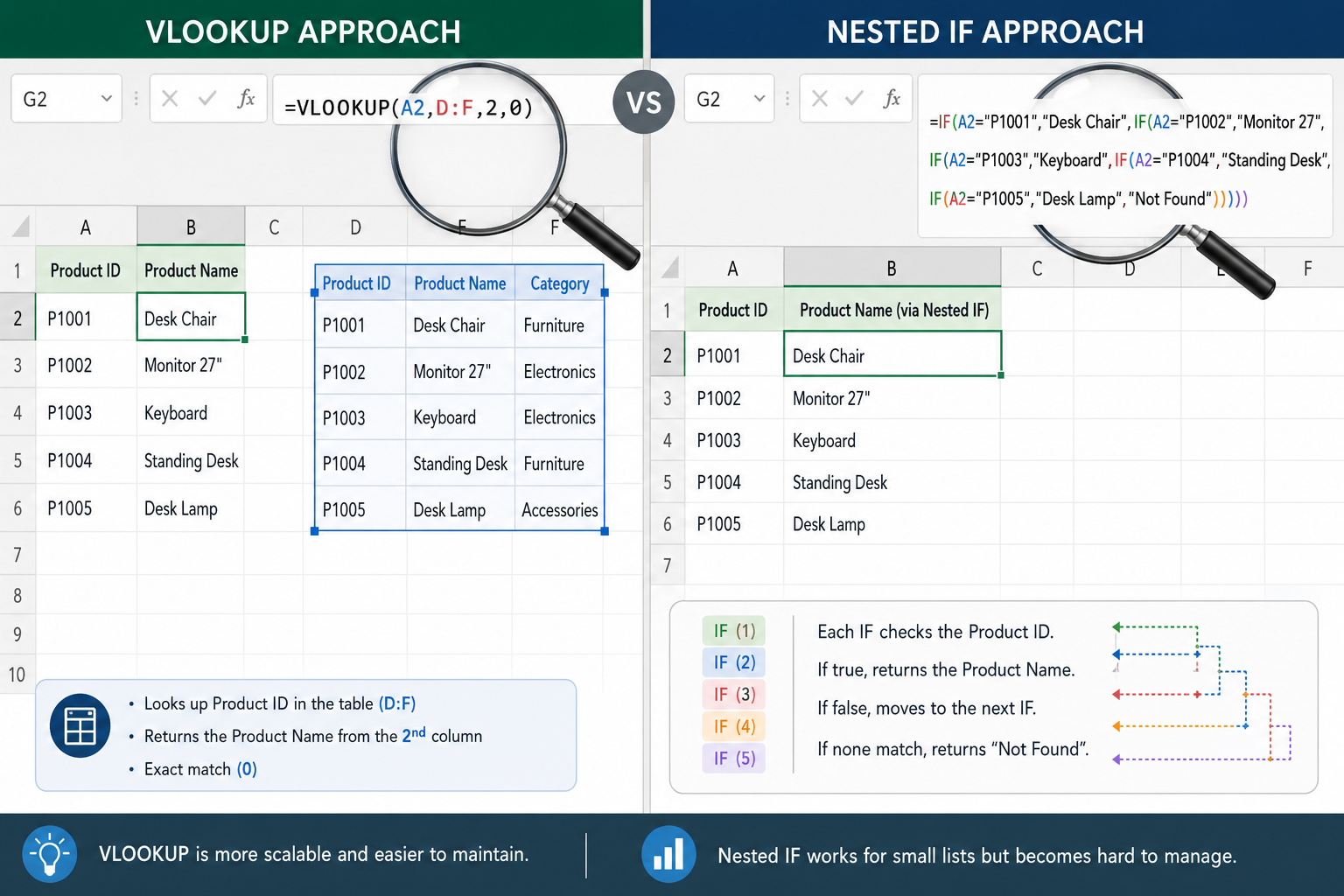
VLOOKUP searches for a value in the first column of a table and returns something from a column to the right. The syntax is: =VLOOKUP(lookup_value, table_range, column_index, [exact_match]). [4]

Step-by-step example:

You have a product list in columns D (ID) and E (Price)
In cell B2, you want the price for the product ID in A2
Write: =VLOOKUP(A2, D:E, 2, 0)
- A2 = what to look up
- D:E = where to look
- 2 = return the 2nd column (Price)
- 0 = exact match

Choose VLOOKUP if your lookup column is on the left side of your table. Choose XLOOKUP (Excel 365/Google Sheets) if you need more flexibility, it can look in any direction: =XLOOKUP(A2, D:D, E:E).

Common mistake: Setting the last argument to 1 (approximate match) when you need an exact match (0). This returns wrong results silently, which is harder to catch than an error.

What's the Easiest Way to Learn VLOOKUP Formulas?

What Are the Most Common Spreadsheet Formula Mistakes Beginners Make?

The most frequent formula errors come from mismatched parentheses, wrong cell references, and mixing text with numbers. Knowing the patterns saves hours of troubleshooting. [9]

Top mistakes and fixes:

Missing the = sign: The formula displays as text. Fix: click the cell, press F2, add = at the start.
Mismatched parentheses: Every open ( needs a closing ). Excel highlights unmatched pairs in color as you type.
Text stored as numbers: If a column of “numbers” won’t sum, check for a green triangle in the corner, the values are text. Use VALUE() to convert, or paste-special as values.
Circular references: A formula that refers to its own cell. Excel warns you, check the formula bar and remove the self-reference.
Hardcoded values inside formulas: Writing =A1*0.08 instead of =A1*$B$1 (where B1 holds the rate) makes future updates painful.

How Do I Fix a Formula That Shows an Error Code?

Each error code in Excel has a specific meaning and a direct fix. Don’t panic, they’re diagnostic messages, not failures. [1]

Error	Cause	Fix
`#DIV/0!`	Dividing by zero or an empty cell	Wrap with `=IFERROR(formula, 0)` or check the divisor
`#VALUE!`	Wrong data type (text where number expected)	Check for text in numeric cells
`#REF!`	A referenced cell was deleted	Re-enter the reference or undo the deletion
`#NAME?`	Misspelled function name	Check spelling; Excel autocomplete helps
`#N/A`	Lookup value not found	Use `IFERROR` or check your lookup table
`#NUM!`	Invalid numeric operation	Check for negative square roots or out-of-range values

Fastest fix for most errors: Wrap the formula in IFERROR: =IFERROR(your_formula, ""), this returns blank (or any message you choose) instead of an ugly error code.

What Formulas Should I Use for Financial Calculations?

For financial work, SUM, AVERAGE, PMT, FV, PV, and IF cover most scenarios. Excel’s financial functions use consistent argument patterns once you learn one. [8]

Most useful financial formulas:

=SUM(B2:B12), total expenses, income, or any running figure
=AVERAGE(B2:B12), monthly average spend
=PMT(rate, nper, pv), monthly loan or mortgage payment. Example: =PMT(5%/12, 60, -20000) gives the monthly payment on a $20,000 loan at 5% over 5 years
=FV(rate, nper, pmt), future value of an investment
=ROUND(A1*1.08, 2), apply tax and round to two decimal places

For a practical example of financial formulas in action, see the Excel Credit Card Payoff Calculator template or the guide to creating a monthly food budget template.

Also useful: the how to round numbers in Excel guide for keeping financial outputs clean.

Are Google Sheets Formulas Different from Excel Formulas?

For most everyday formulas, Google Sheets and Excel are nearly identical, SUM, IF, VLOOKUP, AVERAGE, and COUNTIF work the same way in both. [5] The differences matter mainly at the advanced level.

Key differences:

XLOOKUP and LAMBDA are available in Excel 365 and have been added to Google Sheets, but syntax can vary slightly
Array formulas: In older Excel, you press Ctrl+Shift+Enter to enter an array formula. In Excel 365 and Google Sheets, arrays are automatic (called “dynamic arrays” in Excel)
GOOGLEFINANCE, IMPORTRANGE, QUERY are Google Sheets-only functions with no direct Excel equivalent
Date serial numbers differ slightly between the two, formulas involving dates copied between apps may need adjustment

Bottom line: If you learn formulas in one, you can transfer about 90% of that knowledge to the other.

Which Spreadsheet Program Is Best for Learning Formulas?

Excel is the best choice for learning formulas if you plan to use spreadsheets professionally, because it has the largest function library, the most learning resources, and is the industry standard in finance, operations, and data analysis. Google Sheets is better if you want free, browser-based access and easy collaboration from day one.

Choose Excel if: You work in a corporate environment, need advanced features like Power Query, or want the deepest formula ecosystem
Choose Google Sheets if: You want zero cost, real-time collaboration, or are working on a Chromebook
Both are fine for beginners, the core formula syntax covered in this guide applies to both

New to Excel entirely? The how to use Excel for beginners step by step guide walks through the interface before formulas.

Can I Combine Multiple Formulas Together, and How?

Yes, nesting one formula inside another is standard practice and one of the most powerful things you can do in a spreadsheet. The inner formula runs first and passes its result to the outer formula. [9]

Example, combining IF and SUM: =IF(SUM(B2:B10)>1000, "Over budget", "On track")

This sums B2:B10 first, then IF checks whether the total exceeds 1,000.

Example, combining TEXT and TODAY: =TEXT(TODAY(), "MMMM DD, YYYY"), formats today’s date as “July 06, 2026”

Tips for readable nested formulas:

Build from the inside out, get the inner formula working first
Use the formula bar’s line breaks (Alt+Enter) to visually separate nested levels
Add comments using N(): =SUM(B2:B10)+N("Total sales before tax")

For date-specific formula combinations, see the guide on adding date and time in Excel 365.

How Do I Write Array Formulas and When Would I Need Them?

An array formula processes a range of values in a single step instead of requiring a helper column. In Excel 365 and Google Sheets, most array behavior is automatic, just write the formula normally and it spills results across multiple cells. [10]

Classic use case: Count cells that meet two conditions without COUNTIFS. =SUM((A2:A10="East")*(B2:B10>500)), counts rows where region is “East” AND sales exceed 500.

In older Excel (pre-365), you’d press Ctrl+Shift+Enter to confirm this as an array formula. In Excel 365, just press Enter, it works automatically.

When you actually need array formulas:

Performing calculations across entire columns without helper columns
Returning multiple results from one formula (dynamic arrays)
Using functions like UNIQUE, FILTER, SORT, and SEQUENCE (Excel 365 / Google Sheets)

What’s the Fastest Way to Apply a Formula to Hundreds of Rows?

Double-click the fill handle, the small green square at the bottom-right corner of a selected cell. Excel automatically fills the formula down to the last row of adjacent data. This is faster than dragging and works for hundreds or thousands of rows instantly. [3]

Other fast methods:

Ctrl+D: Select the formula cell plus the cells below it, then press Ctrl+D to fill down
Copy and paste: Copy the formula cell (Ctrl+C), select the destination range, paste (Ctrl+V)
Name a Table: Convert your data to an Excel Table (Ctrl+T), any formula added to a column automatically fills to every row, including new rows added later

✅ Best practice for large datasets: Use Excel Tables. They’re the most reliable way to ensure formulas stay consistent as data grows.

Do I Need to Memorize All Formulas, or Can I Look Them Up?

No, you do not need to memorize formulas. Professional spreadsheet users look up syntax regularly, and Excel’s built-in tools make this easy. [9]

Built-in help tools:

Autocomplete: Start typing =SU and Excel shows a dropdown of matching functions
Function Wizard: Click the fx button next to the formula bar for guided argument entry
Formula tooltips: Once you type a function name and (, Excel shows the argument structure inline
Insert Function dialog: Shift+F3 opens a searchable list of all available functions

What’s worth memorizing: The 10-15 functions you use every week (SUM, IF, VLOOKUP/XLOOKUP, COUNTIF, SUMIF, AVERAGE, TEXT, IFERROR, LEFT/RIGHT/MID). Everything else, look up as needed.

For a quick reference sheet, the 50 time-saving keyboard shortcuts for Excel guide pairs well with formula practice.

FAQ

Q: Why does my formula show the formula text instead of a result? The cell is formatted as Text, or the = sign is missing. Click the cell, change the format to General, press F2, then Enter.

Q: Can I use a formula across multiple sheets? Yes. Reference another sheet with the syntax =SheetName!A1. For example, =Sales!B10 pulls the value from cell B10 on the “Sales” sheet.

Q: What’s the difference between SUMIF and SUMIFS? SUMIF handles one condition; SUMIFS handles multiple. Example: =SUMIFS(C:C, A:A, "East", B:B, ">500") sums column C where A is “East” and B exceeds 500.

Q: How do I count cells that contain text? Use =COUNTA(A1:A100) to count non-empty cells, or =COUNTIF(A1:A100, "*") to count cells containing any text.

Q: What does the & operator do in a formula? It joins (concatenates) text. =A1&" "&B1 combines the first and last name from two cells with a space between them.

Q: How do I stop a formula from recalculating every time I open the file? Go to Formulas > Calculation Options > Manual. Press F9 to recalculate on demand. Use this for very large files that slow down on auto-calculate.

Q: What’s the fastest way to see all formulas in a spreadsheet at once? Press Ctrl+` (grave accent) to toggle formula view on and off. Every cell shows its formula instead of its result.

Q: Is XLOOKUP better than VLOOKUP? For most tasks, yes. XLOOKUP is more flexible (searches any direction), handles missing values more cleanly, and doesn’t require counting column numbers. Use XLOOKUP in Excel 365 or Google Sheets when available.

Q: How do I reference a whole column without slowing down the file? In Excel, A:A references the entire column but can slow calculation in large files. Use a defined range like A2:A10000 or an Excel Table reference instead.

Q: Can formulas pull data from another file? Yes, in Excel: =[Workbook.xlsx]Sheet1!A1. Note that external links require the source file to be open or accessible for the formula to update.

Conclusion

Writing spreadsheet formulas is a learnable skill, not a talent, and this How to Write Spreadsheet Formulas: A Beginner-to-Advanced Guide covers everything from the first =SUM to nested IFs and dynamic arrays. The logic behind formulas matters more than memorizing syntax: understand cell references, operators, and function structure, and you can figure out almost any formula from there.

Actionable next steps:

Open a blank spreadsheet and practice the five core formulas: SUM, AVERAGE, IF, VLOOKUP, and COUNTIF
Convert your next data range into an Excel Table (Ctrl+T) to make formula management automatic
Bookmark the function autocomplete, let Excel guide you rather than memorizing syntax cold
When a formula breaks, read the error code first, each one points directly to the problem
Explore the how to use Excel step by step PDF for a printable reference to keep beside your keyboard

The best formula writers aren’t the ones who know the most functions, they’re the ones who understand the logic well enough to build what they need, one step at a time.

References

[1] Overview Of Formulas In Excel – https://support.microsoft.com/en-us/excel/get-started/overview-of-formulas-in-excel [2] Create A Simple Formula In Excel – https://support.microsoft.com/en-us/office/create-a-simple-formula-in-excel-11a5f0e5-38a3-4115-85bc-f4a465f64a8a [3] Creating and Editing Formulas – https://support.spreadsheet.com/hc/en-us/articles/360030711652-Creating-and-Editing-Formulas [4] Examples Of Commonly Used Formulas – https://support.microsoft.com/en-us/office/examples-of-commonly-used-formulas-b45a3946-819e-455e-ac20-770ea6aa05da [5] Formulae With Spreadsheets – https://okfnlabs.org/handbook/data/patterns/formulae-with-spreadsheets/ [8] Excel Formulas Cheat Sheet – https://corporatefinanceinstitute.com/resources/excel/excel-formulas-cheat-sheet/ [9] Mastering Excel Formula Writing: A Step By Step Guide – https://ajelix.com/excel/mastering-excel-formula-writing-a-step-by-step-guide/ [10] Excel Advanced Formulas: XLOOKUP, LAMBDA, Arrays – https://indigosoftwarecompany.com/excel-advanced-formulas-xlookup-lambda-arrays/