Last updated: June 24, 2026
Quick Answer: To freeze a row in Excel, click the View tab on the ribbon, select Freeze Panes, then choose Freeze Top Row to lock the first row in place. For multiple rows, click the row below the last row you want frozen, then choose Freeze Panes from the same menu. The frozen row stays visible as you scroll down through your data.
Key Takeaways
- Freeze Top Row locks only row 1 — the fastest option for most spreadsheets with a single header row.
- To freeze multiple rows, select the row below the last row you want frozen before applying Freeze Panes.
- You can freeze rows and columns at the same time by clicking a cell (not just a row or column) before applying Freeze Panes.
- The Freeze Panes option lives under the View tab in Excel on both Windows and Mac.
- Freezing a row does not affect printing — use Page Layout > Print Titles to repeat rows on printed pages.
- Only one freeze pane can be active at a time; applying a new freeze replaces the old one.
- To remove frozen panes, go to View > Freeze Panes > Unfreeze Panes.
- Frozen rows are purely visual — they don’t lock cells from editing (that’s a separate protection feature).
Why Freezing a Row in Excel Matters
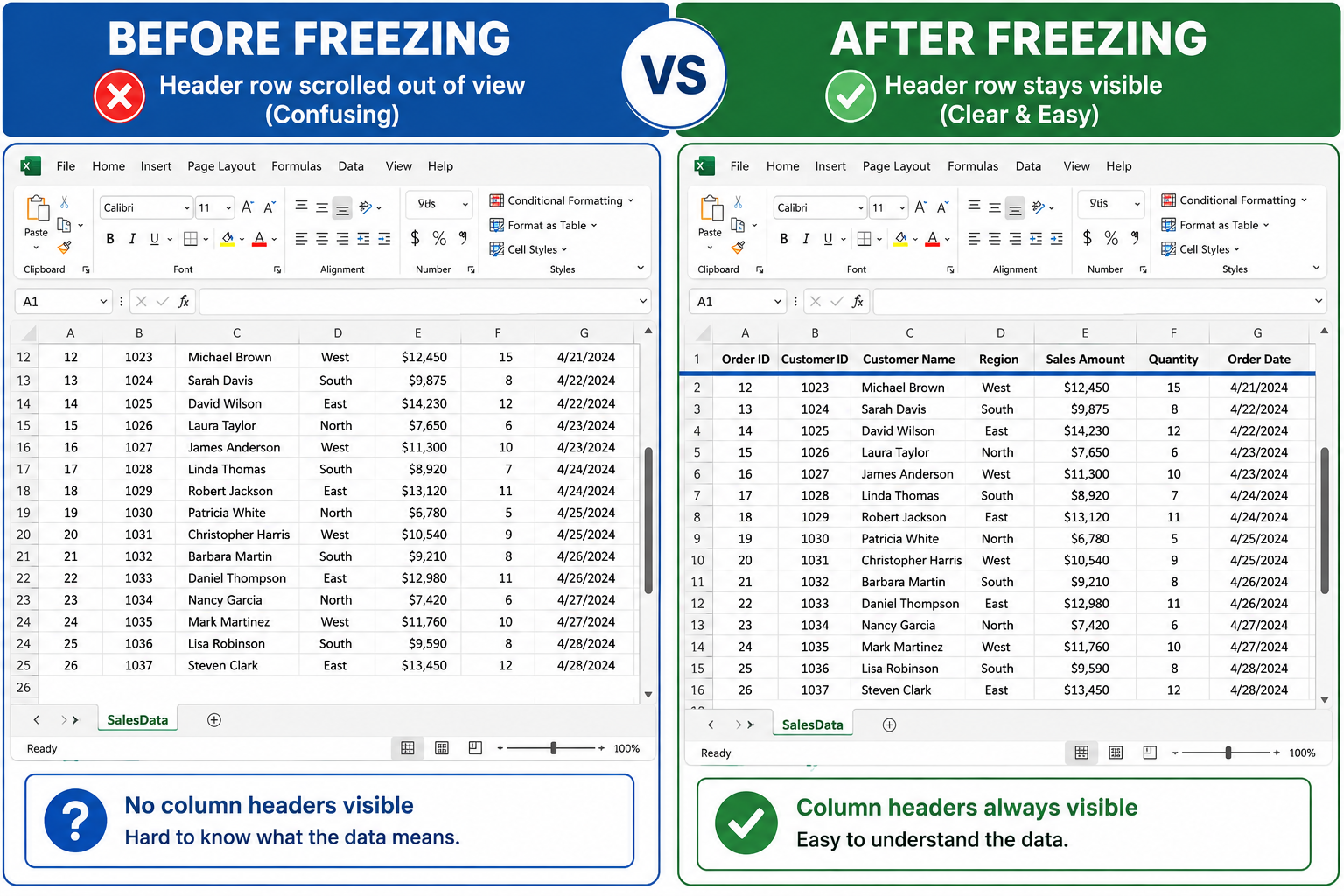
Scrolling through a large dataset and losing track of your column headers is one of the most common Excel frustrations. Knowing how to freeze a row in Excel solves this instantly — your header row stays pinned at the top no matter how far down you scroll. [4]
This feature is called Freeze Panes, and it’s been a core part of Excel for decades. It works across Excel 365, Excel 2021, Excel 2019, Excel 2016, and Excel for Mac. [2]
Who benefits most:
- Anyone working with spreadsheets longer than one screen
- Budget trackers, project managers, and data analysts
- Students building their first structured dataset (a college budget template is a perfect example)
- Anyone sharing files with colleagues who need clear, readable data
How to Freeze the Top Row in Excel (Quickest Method)
This is the most common use case: you have a single header row at the top and want it to stay visible as you scroll. [3]
Steps:
- Open your Excel workbook.
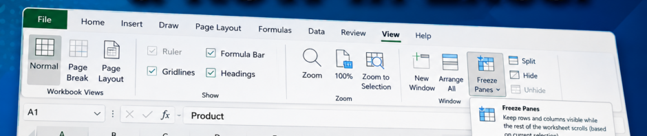
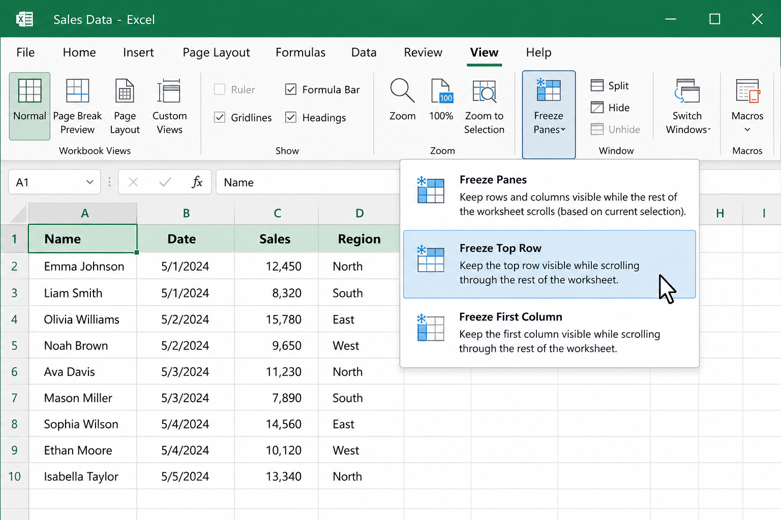
- Click the View tab on the ribbon.
- Click Freeze Panes in the Window group.
- Select Freeze Top Row from the dropdown.
A thin gray or blue line appears below row 1, confirming the freeze is active. Scroll down — row 1 stays locked. [4]
Common mistake: Clicking a cell before selecting “Freeze Top Row” doesn’t matter here — Excel always freezes row 1 with this option regardless of which cell is selected. [5]
How to Freeze Multiple Rows in Excel
When your spreadsheet has two or more header rows (for example, a title row plus a column label row), you need to freeze all of them together.
Steps:
- Click on the row number of the row directly below the last row you want frozen. For example, to freeze rows 1 and 2, click on row 3’s row number to select the entire row.
- Go to View > Freeze Panes > Freeze Panes (the first option in the list, not “Freeze Top Row”).
- A freeze line appears below row 2, locking both rows in place. [6]
Choose this method if: Your spreadsheet has a title in row 1 and column headers in row 2, or if you’re working with grouped header structures.
Edge case: If you select a cell in column B or further right instead of selecting the full row, Excel may freeze both rows and columns simultaneously. To freeze rows only, click the row number on the far left to select the entire row first. [7]
How to Freeze Rows and Columns at the Same Time
Freezing both rows and columns at once keeps your headers and your row labels visible no matter where you scroll — useful for large financial models or comparison tables.
Steps:
- Click the cell that sits directly below the rows you want frozen and directly to the right of the columns you want frozen. For example, to freeze row 1 and column A, click cell B2.
- Go to View > Freeze Panes > Freeze Panes.
- Freeze lines appear both below row 1 and to the right of column A. [4]
| Goal | Click Here First | Then Choose |
|---|---|---|
| Freeze top row only | Any cell | Freeze Top Row |
| Freeze first column only | Any cell | Freeze First Column |
| Freeze rows 1 & 2 | Row 3 (entire row) | Freeze Panes |
| Freeze row 1 + column A | Cell B2 | Freeze Panes |
| Freeze rows 1–3 + columns A–B | Cell C4 | Freeze Panes |
How to Freeze a Row in Excel on a Mac
The process for freezing rows on Excel for Mac is nearly identical to Windows, with one small difference in where the menu lives. [2]
Steps (Excel for Mac):
- Click the View tab in the top menu bar.
- Click Freeze Panes.
- Choose Freeze Top Row, Freeze First Column, or Freeze Panes depending on your need.
The keyboard shortcut path on Mac: View menu > Freeze Panes (there’s no single keyboard shortcut by default, but you can assign one in System Preferences). [2]
For more keyboard-driven workflows, check out these Excel shortcut keys that can speed up your everyday tasks.
How to Unfreeze Rows in Excel
Unfreezing is just as simple as freezing. Go to View > Freeze Panes > Unfreeze Panes. The option only appears when a freeze is already active — if you don’t see it, no freeze is currently applied. [3]
Note: You can’t selectively unfreeze one row while keeping another frozen. Unfreeze Panes removes all active freeze panes at once. To change which rows are frozen, unfreeze first, then reapply with the new selection.
Freeze Panes vs. Split Panes: What’s the Difference?
Both features help you view different parts of a spreadsheet at once, but they work differently.
- Freeze Panes: Locks specific rows or columns so they stay visible while the rest of the sheet scrolls. The frozen section can’t be scrolled independently.
- Split Panes: Divides the Excel window into separate scrollable sections. Each section can scroll independently. Found under View > Split.
Choose Freeze Panes if you want a persistent header row that stays put. Choose Split if you need to compare two distant parts of the same sheet side by side.
This pairs well with other display tips — for example, learning how to merge cells in Excel using shortcut keys can help you build cleaner header structures before you freeze them.
Common Mistakes When Freezing Rows (and How to Fix Them)
Even a simple feature like Freeze Panes has a few traps worth knowing about.
Mistake 1: Applying Freeze Panes from the wrong cell If you click a random cell in the middle of your sheet and choose “Freeze Panes,” Excel freezes everything above and to the left of that cell — not just the top row. Always check where your cursor is before applying. [5]
Mistake 2: Expecting frozen rows to print Freeze Panes is a display-only feature. To repeat rows on every printed page, go to Page Layout > Print Titles > Rows to repeat at top. [4]
Mistake 3: Confusing freezing with cell protection Frozen rows are still fully editable. If you need to prevent edits to specific cells, that’s a separate process — explore how to lock specific cells in Excel for that workflow.
Mistake 4: Trying to freeze a row in the middle of the sheet Freeze Panes always freezes from the top (or left) edge of the sheet. You can’t freeze row 5 while leaving rows 1–4 scrollable. If you need that kind of navigation, consider filtering or using Excel Tables instead.
Tips for Working With Frozen Rows in Large Spreadsheets
Once your rows are frozen, a few extra habits make large spreadsheets much easier to manage.
- Use Excel Tables (Ctrl+T): Converting your data range to a Table automatically keeps column headers visible in the column letter area when you scroll — even without Freeze Panes. It’s a useful backup.
- Color your header row: A distinct header color makes the frozen row visually obvious. Check out how to apply color to alternate rows using conditional formatting for a polished look.
- Combine with hiding columns: If your sheet is wide, hiding columns you don’t need reduces horizontal scrolling. See these tips on hiding columns with keyboard shortcuts.
- Wrap text in headers: Long header labels can be hard to read. Wrapping text in Excel keeps the frozen row compact and readable.
FAQ
Q: Can you freeze a row in Excel Online (browser version)? A: Yes. In Excel Online, go to View > Freeze Rows & Columns and choose your option. The interface is slightly different but the result is the same.
Q: Does freezing rows slow down Excel? A: No. Freeze Panes is a display setting with no meaningful impact on spreadsheet performance.
Q: Can you freeze the bottom row instead of the top? A: No. Excel’s Freeze Panes only works from the top and left edges. There’s no built-in option to freeze the bottom row.
Q: Why is “Freeze Panes” grayed out? A: This usually happens when the sheet is in cell editing mode or when the workbook is protected. Press Escape to exit editing mode, or check if the workbook has protection applied.
Q: Does Freeze Panes work in Excel for iPad or iPhone? A: Yes, though the option is found under View in the mobile ribbon. The steps are the same as desktop.
Q: How many rows can you freeze at once? A: There’s no hard limit, but freezing many rows reduces the visible scrollable area. Practically, most users freeze 1–3 rows.
Q: Will frozen rows stay when I share the file? A: Yes. The freeze setting is saved with the workbook, so anyone who opens the file will see the same frozen rows — as long as they’re using a version of Excel that supports it.
Q: Can I freeze rows in a protected sheet? A: Only if the sheet protection settings allow it. By default, protection locks the freeze state in place, which can actually be useful for shared templates.
Conclusion
Knowing how to freeze a row in Excel is one of those small skills that pays off every single day. Whether you’re managing a simple budget or a complex dataset with hundreds of rows, keeping your headers visible makes the whole experience faster and less error-prone.
Your next steps:
- Open any Excel spreadsheet with a header row.
- Click View > Freeze Panes > Freeze Top Row — takes under five seconds.
- Scroll down and confirm the header stays locked.
- If you need to freeze multiple rows, click the row below your headers first, then choose Freeze Panes.
- Explore related formatting improvements like conditional formatting for alternate rows or wrapping text in headers to make your frozen rows even cleaner.
Once it’s set up, you’ll wonder how you ever scrolled through a long spreadsheet without it.
References
[2] Freeze Panes To Lock The First Row Or Column In Excel For Mac – https://support.microsoft.com/en-us/excel/freeze-panes-to-lock-the-first-row-or-column-in-excel-for-mac
[3] How To Freeze A Row In Excel – https://www.xelplus.com/how-to-freeze-a-row-in-excel/
[4] Freeze Panes To Lock Rows And Columns – https://support.microsoft.com/en-us/office/freeze-panes-to-lock-rows-and-columns-dab2ffc9-020d-4026-8121-67dd25f2508f
[5] Excel How To Freeze Rows – https://www.excel-university.com/excel-how-to-freeze-rows/
[6] Freezing Excel Rows – https://www.ionos.com/digitalguide/online-marketing/online-sales/freezing-excel-rows/
[7] Freeze Panes Excel – https://www.goskills.com/excel/resources/freeze-panes-excel
[10] Freeze Cells In Excel – https://www.wikihow.com/Freeze-Cells-in-Excel