
Click here to view our video tutorial.
Click here to download our PDF tutorial.
How to Remove or Hide Numbers After the Decimal in Excel (Step-by-Step Guide)

If you work with numbers in Excel, you may often find decimal places getting in the way of clean, easy-to-read data. Whether you’re preparing a report, simplifying spreadsheet visuals, or just trying to get whole numbers for calculations, removing or hiding decimals can make your sheet more effective.
In this guide, you’ll learn three easy methods to either completely remove or simply hide the numbers after the decimal in Excel. We’ll walk through each method step-by-step, using visuals for every stage.
Here’s What We’ll Cover:
- How to use the Formulas tab to insert the TRUNC function without typing.
- How to hide numbers after the decimal using Format Cells.
- How to quickly hide numbers after the decimal using the Decrease Decimal button.
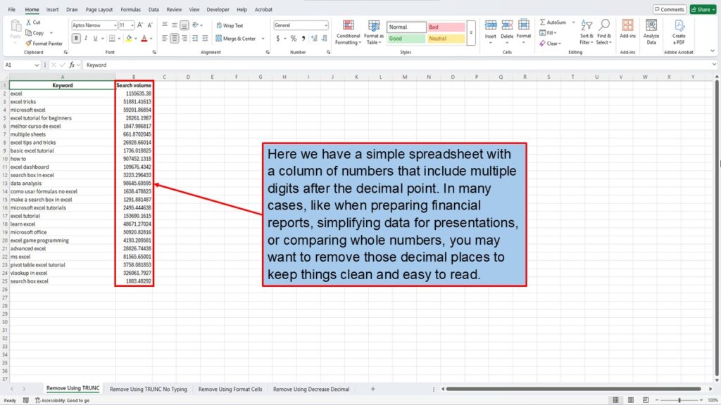
Here we have a simple spreadsheet with a column of numbers that include multiple digits after the decimal point. In many cases, like when preparing financial reports, simplifying data for presentations, or comparing whole numbers, you may want to remove those decimal places to keep things clean and easy to read.
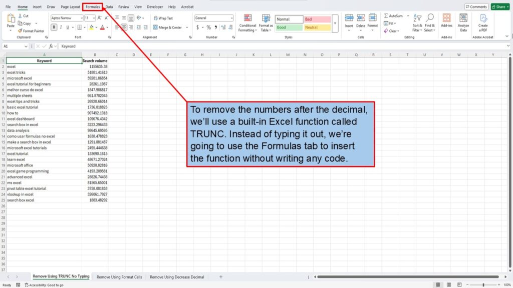
To remove the numbers after the decimal, we’ll use a built-in Excel function called TRUNC. Instead of typing it out, we’re going to use the Formulas tab to insert the function without writing any code.
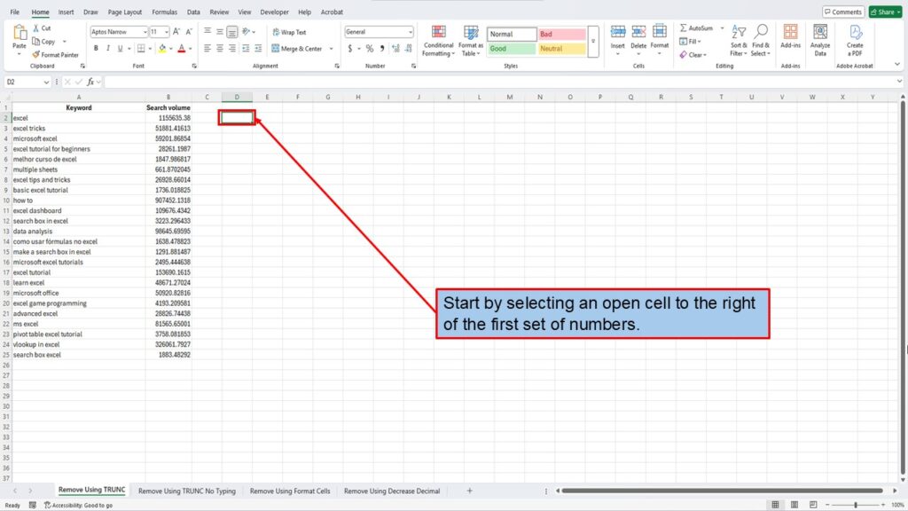
Start by selecting an open cell to the right of the first set of numbers.
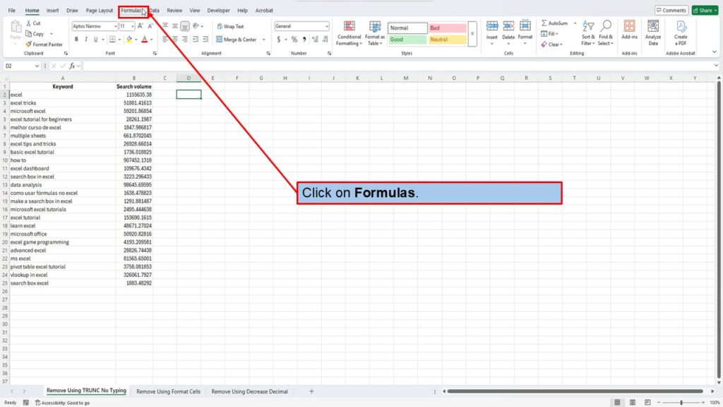
Click on Formulas.
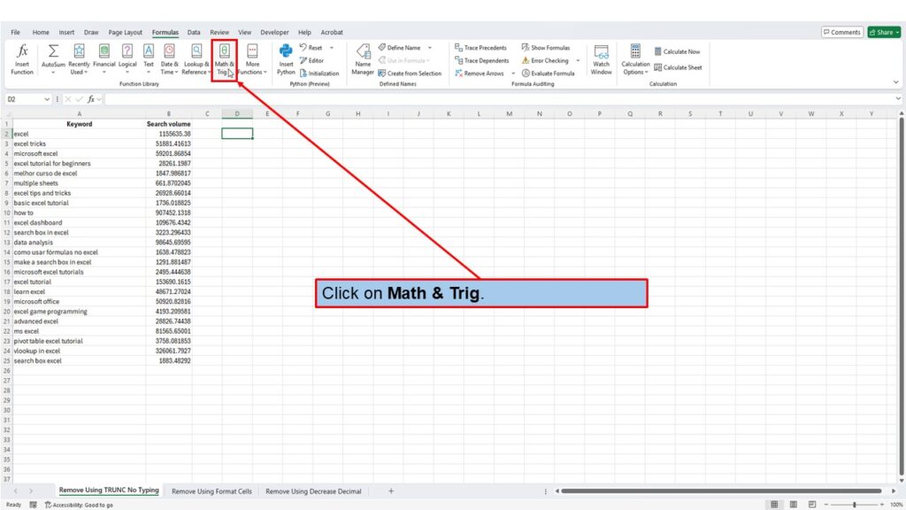
Click on Math & Trig.
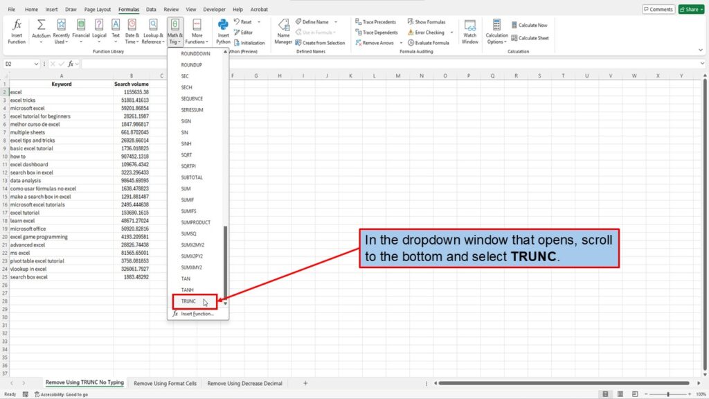
In the dropdown window that opens, scroll to the bottom and select TRUNC.
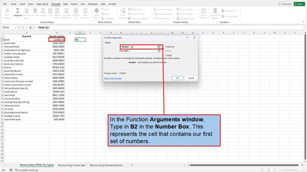
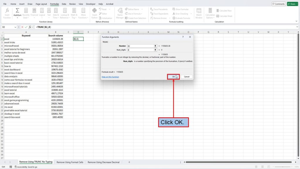
In the Function Arguments window, type in B2 in the Number box. This represents the cell that contains our first set of numbers.
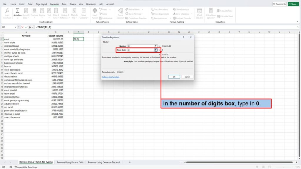
In the number of digits box, type in 0.
Click OK.
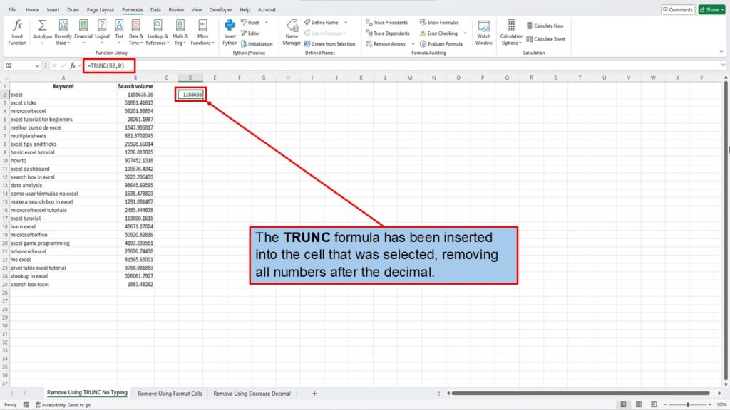
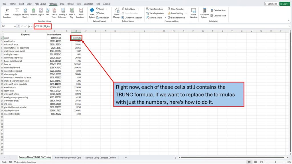
The TRUNC formula has been inserted into the cell that was selected, removing all numbers after the decimal.
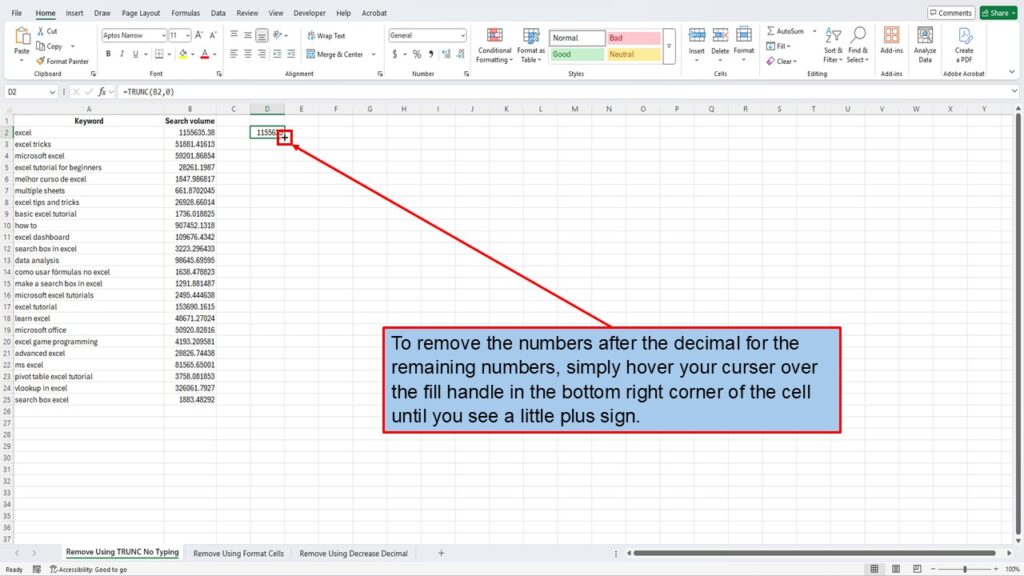
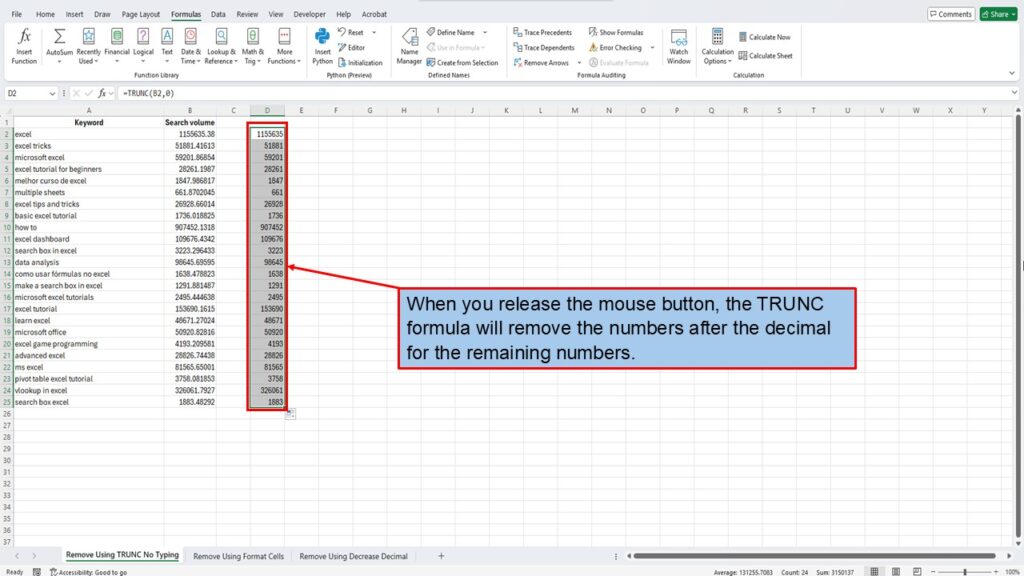
To remove the numbers after the decimal for the remaining numbers, simply hover your cursor over the fill handle in the bottom right corner of the cell until you see a little plus sign.
Left-click and drag the cell down.
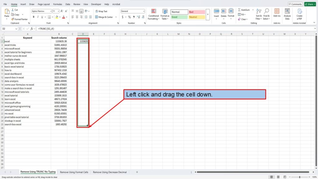
When you release the mouse button, the TRUNC formula will remove the numbers after the decimal for the remaining numbers.
Right now, each of these cells still contains the TRUNC formula. If we want to replace the formulas with just the numbers, here’s how to do it.
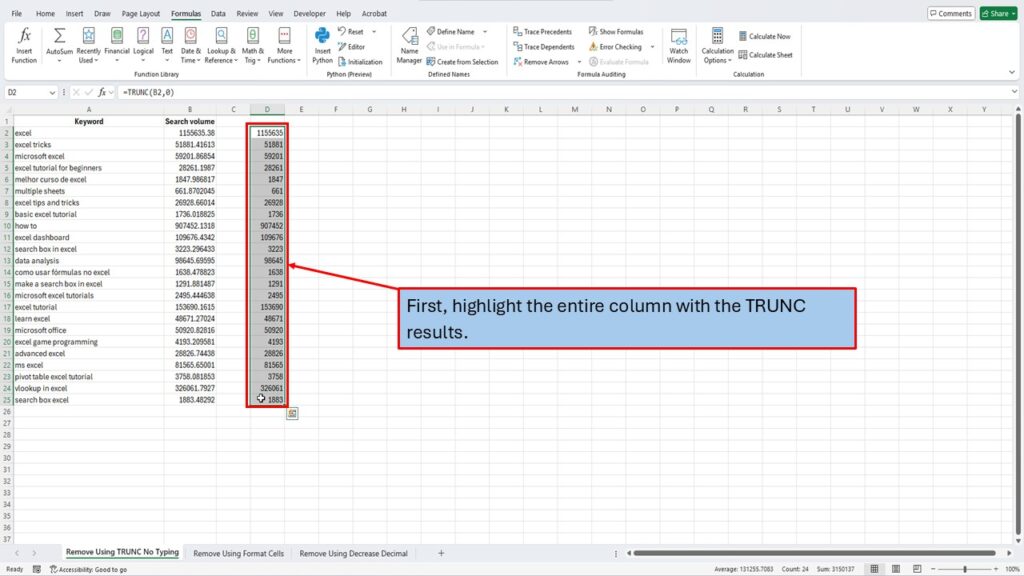
First, highlight the entire column with the TRUNC results.
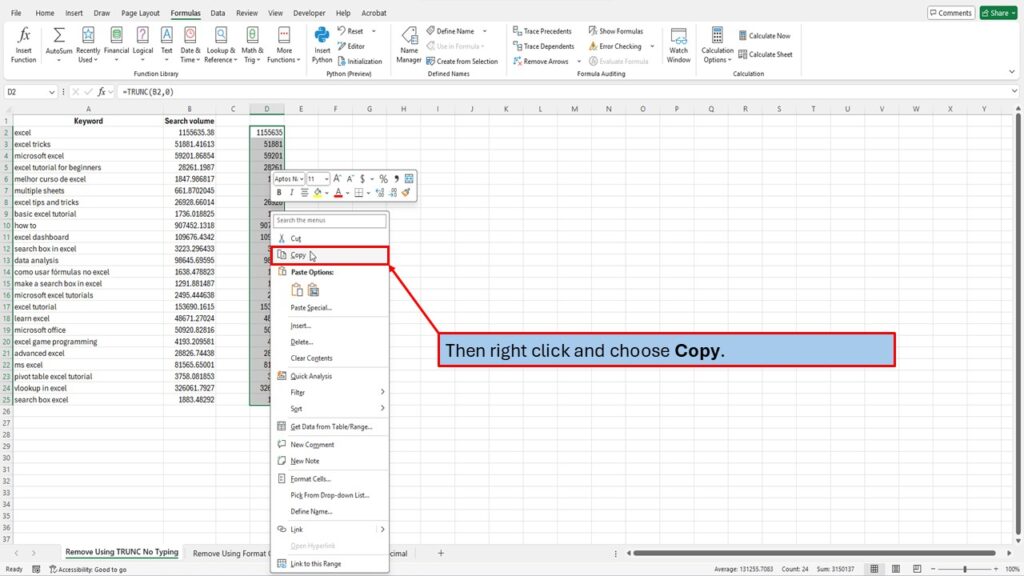
Then right-click and choose Copy.
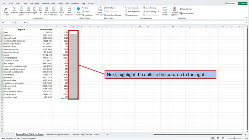
Next, highlight the cells in the column to the right.
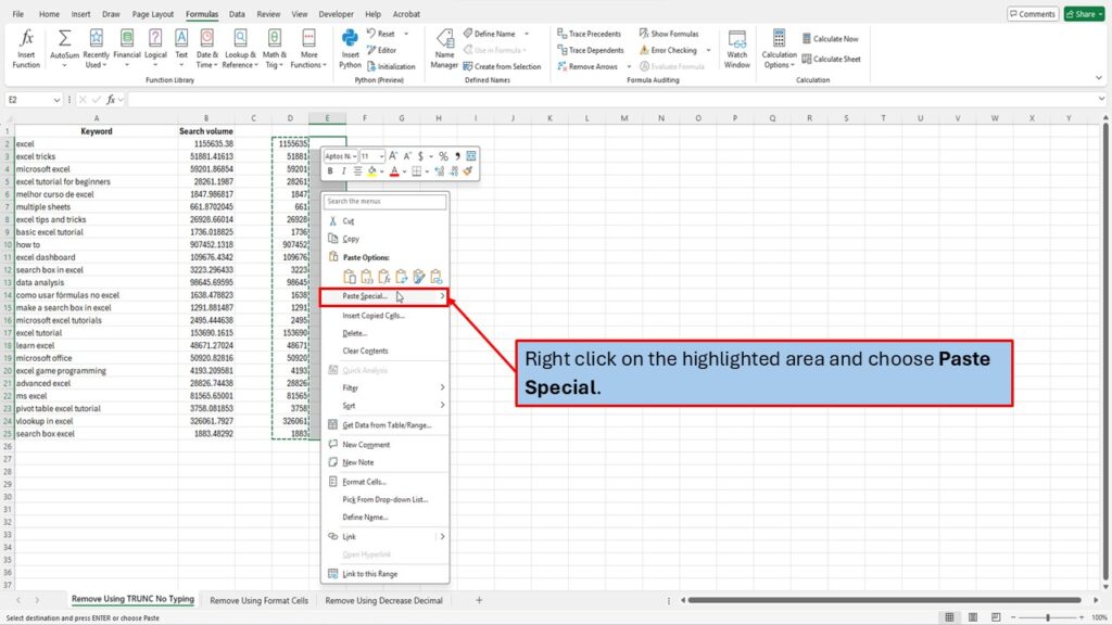
Right-click on the highlighted area and choose Paste Special.
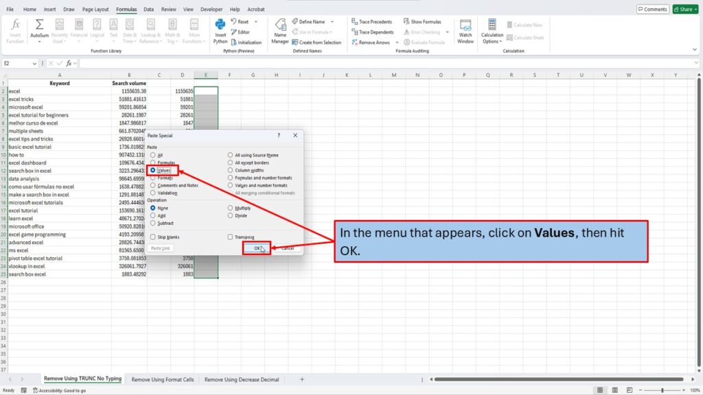
In the menu that appears, click on Values, then hit OK.
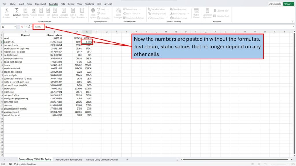
Now the numbers are pasted in without the formulas—just clean, static values that no longer depend on any other cells.
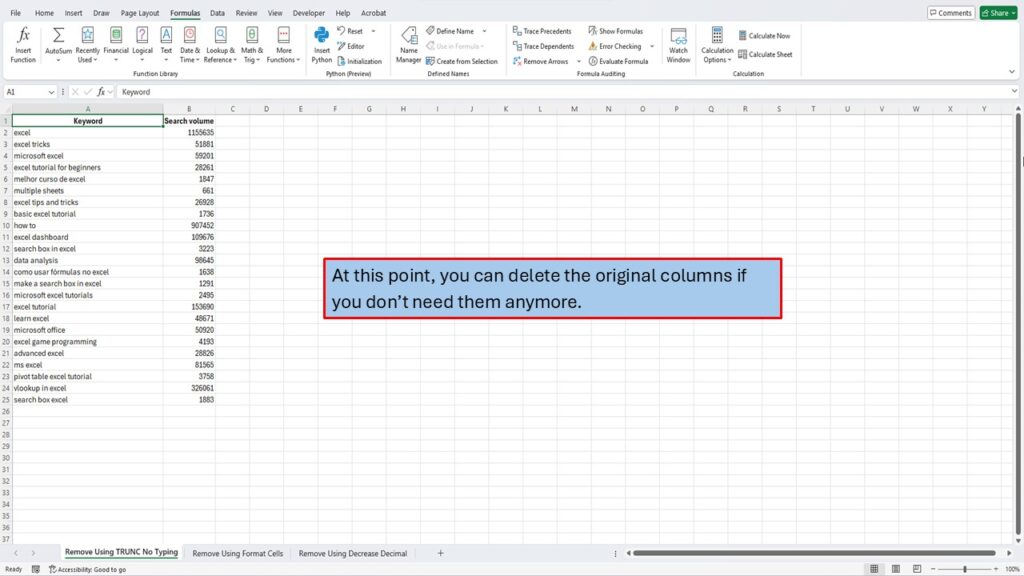
At this point, you can delete the original columns if you don’t need them anymore.
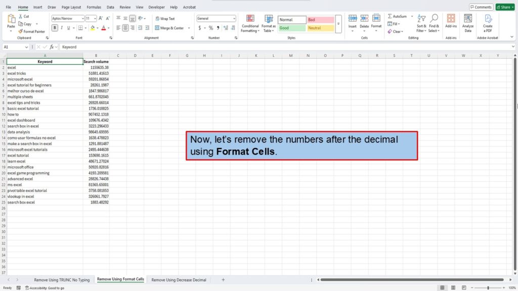
Now, let’s remove the numbers after the decimal using Format Cells.
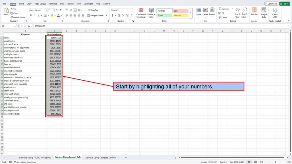
Start by highlighting all of your numbers.
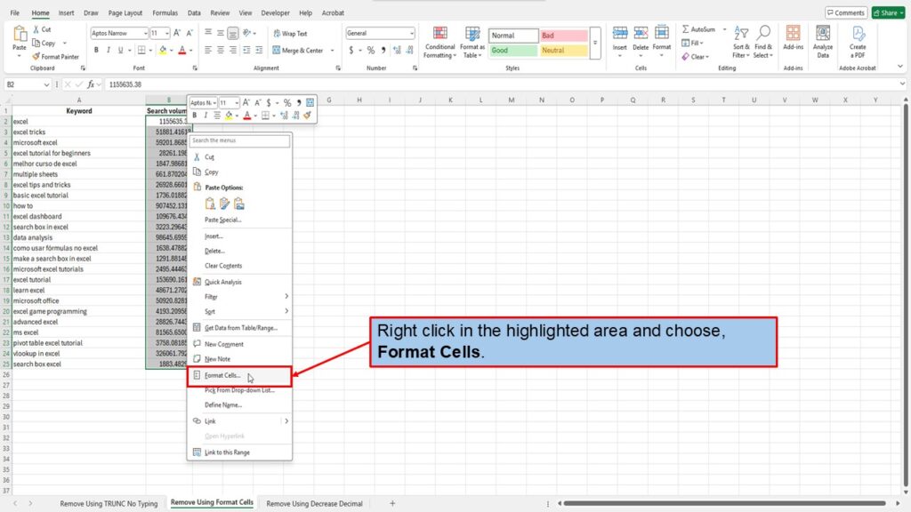
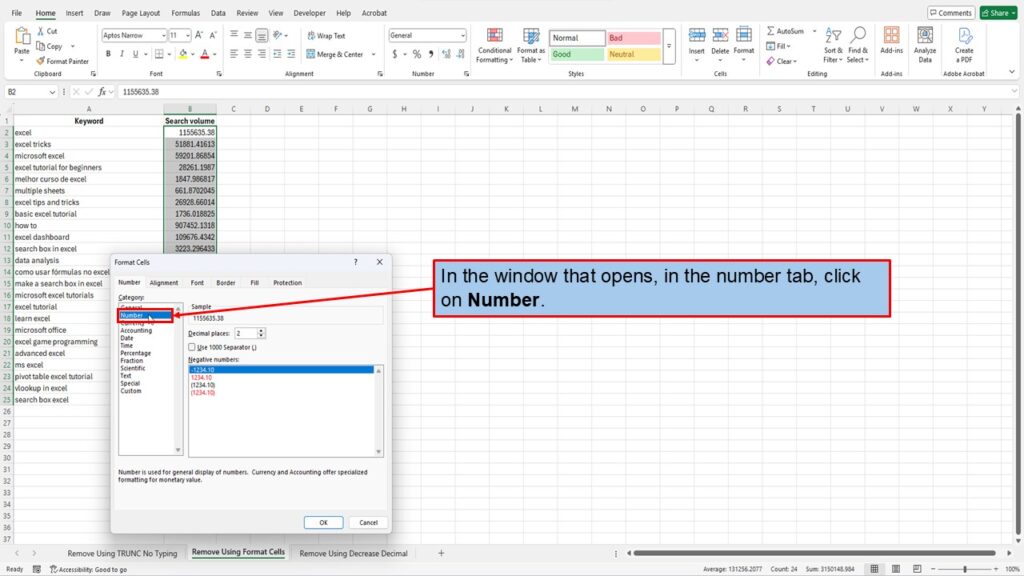
Right-click in the highlighted area and choose Format Cells.
In the window that opens, in the Number tab, click on Number.
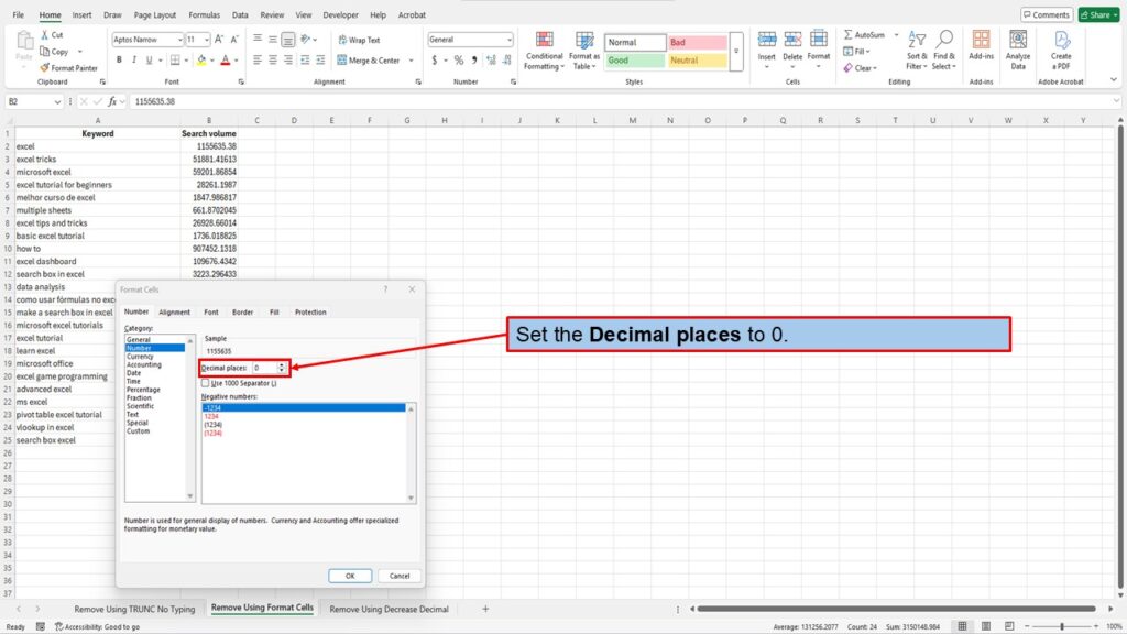
Set the Decimal Places to 0.
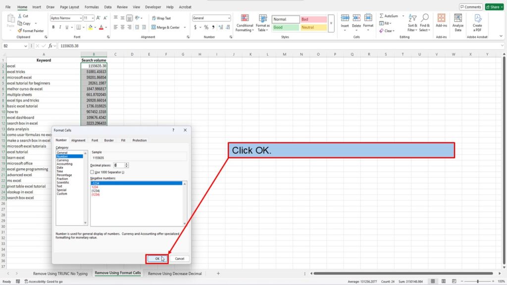
Click OK.
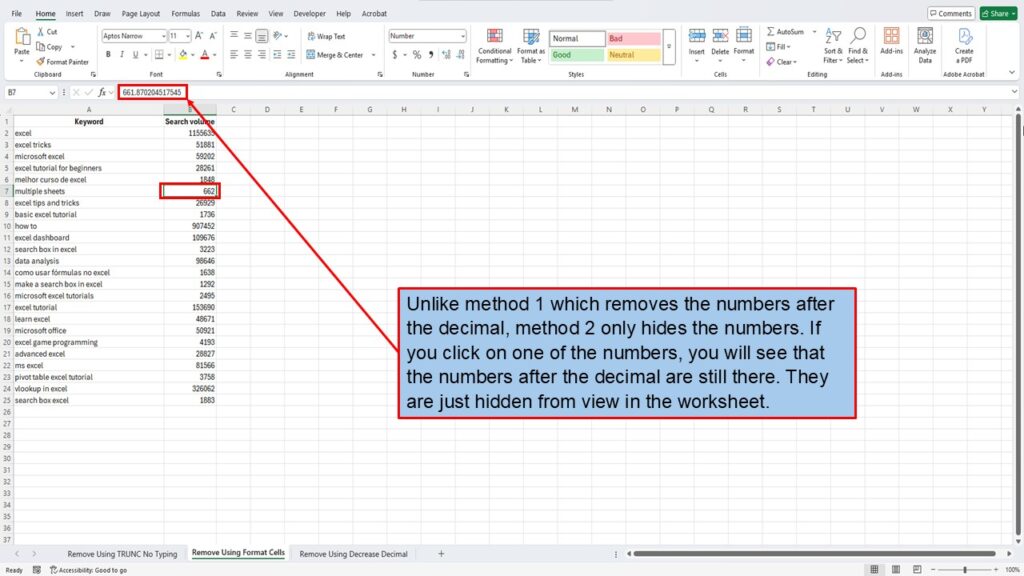
The numbers after the decimal have been removed.
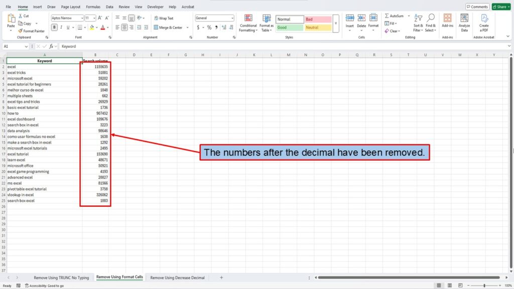
Unlike Method 1 which removes the numbers after the decimal, Method 2 only hides the numbers. If you click on one of the numbers, you will see that the numbers after the decimal are still there. They are just hidden from view in the worksheet.
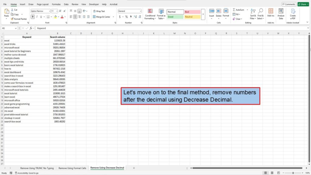
Let’s move on to the final method: remove numbers after the decimal using Decrease Decimal.
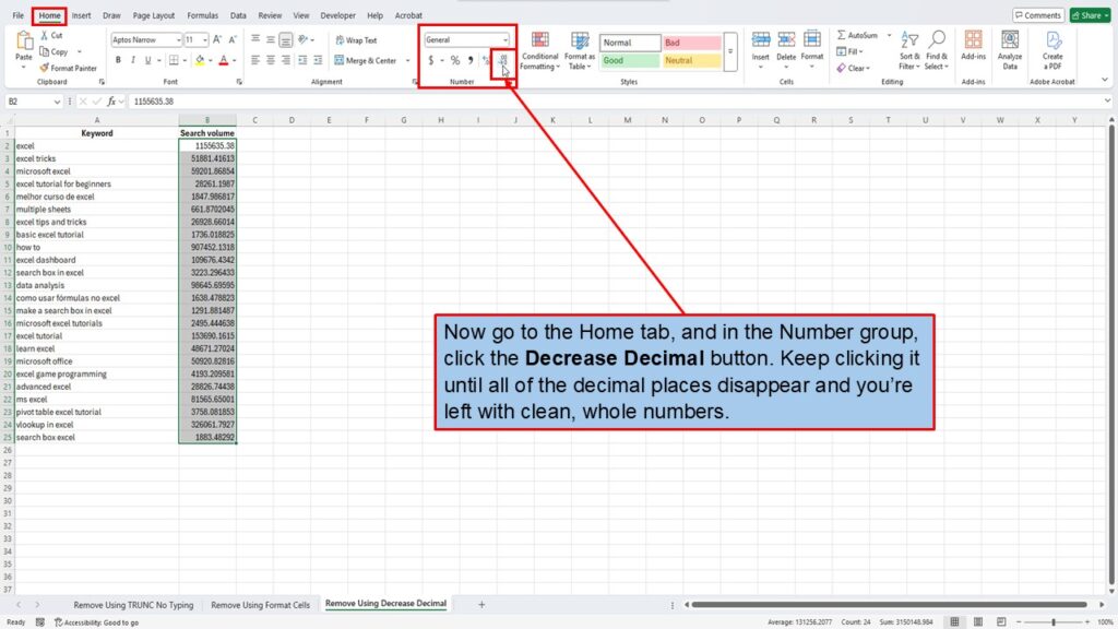
Start by highlighting your numbers.

Now go to the Home tab, and in the Number group, click the Decrease Decimal button. Keep clicking it until all of the decimal places disappear and you’re left with clean, whole numbers.
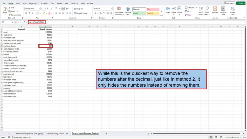
While this is the quickest way to remove the numbers after the decimal, just like in Method 2, it only hides the numbers instead of removing them.
Conclusion
Removing or hiding decimals in Excel doesn’t have to be complicated. If you need to fully remove the decimal values, the TRUNC function is your best option. If you just want to hide them for cleaner visuals, Format Cells or Decrease Decimal will do the trick.
Choose the method that fits your needs best—whether you’re simplifying a report, creating charts, or sharing a cleaner dataset with others.
If this guide helped you, be sure to check out our other Excel tutorials for more practical tips!
Need More Help?
Video Tutorial
Download PDF Below
Check Out My Latest Post: How to Remove Conditional Formatting in Excel (Entire Worksheet)
Visit My YouTube Channel.