
Locking cells in Excel is a fundamental skill that ensures the integrity of your data by preventing unintended modifications.
By default, all cells in an Excel worksheet are locked, but this setting only takes effect when the worksheet is protected.
This guide provides a comprehensive, step-by-step approach to locking specific cells, offering detailed explanations to enhance your understanding.
Click here to view our video tutorial.
Click here to download our PDF tutorial.
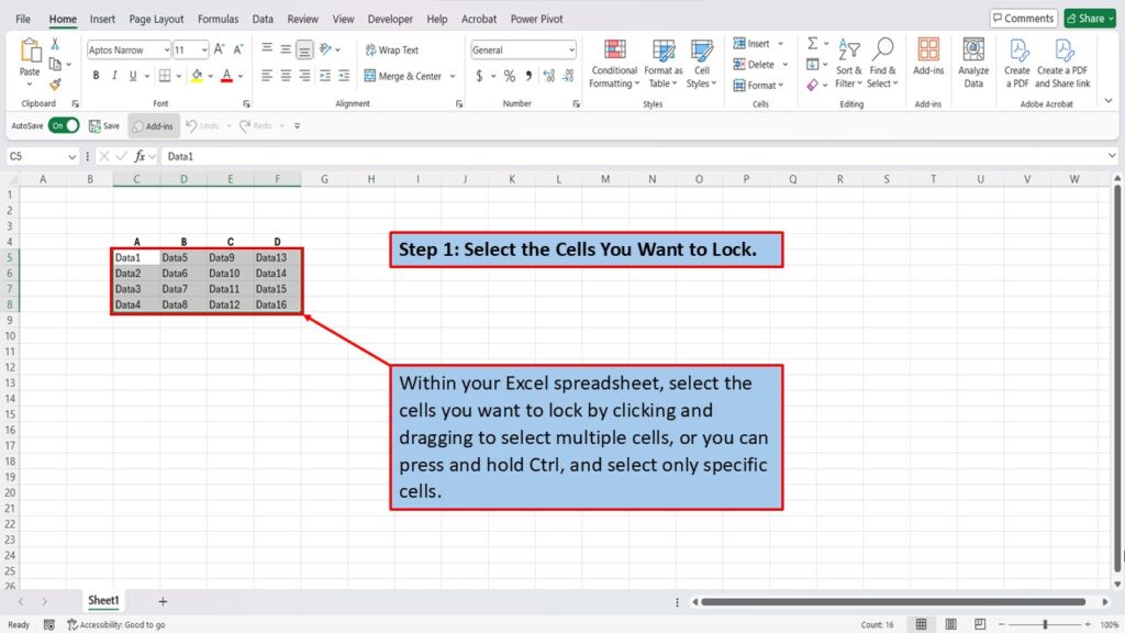
Step 1: Select the Cells You Want to Lock.
Begin by identifying the cells that you want to protect from editing. To select multiple cells:
Non-Adjacent Cells: Hold down the Ctrl key and click on each cell you wish to select.
Adjacent Cells: Click and drag your mouse over the desired cells.
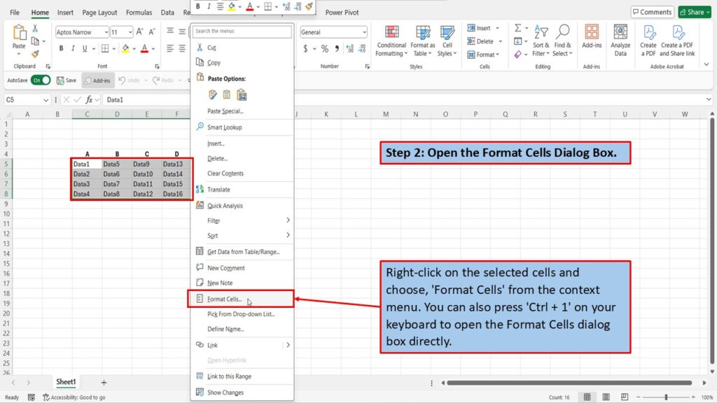
Step 2: Open the Format Cells Dialog Box.
Once your desired cells are selected:
Keyboard Shortcut: Press Ctrl + 1 to open the Format Cells dialog box directly.
Right-Click Method: Right-click on any of the selected cells and choose ‘Format Cells’ from the context menu.
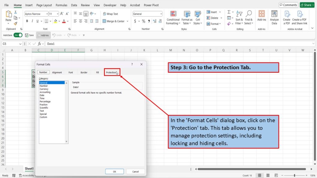
Step 3: Go to the Protection Tab.
In the Format Cells dialog box:
Hidden: Conceals the cell’s content in the formula bar when the cell is selected, provided the worksheet is protected.
Click on the ‘Protection’ tab.
Here, you’ll see two options: ‘Locked’ and ‘Hidden’.
Locked: Prevents users from editing the cell when the worksheet is protected.
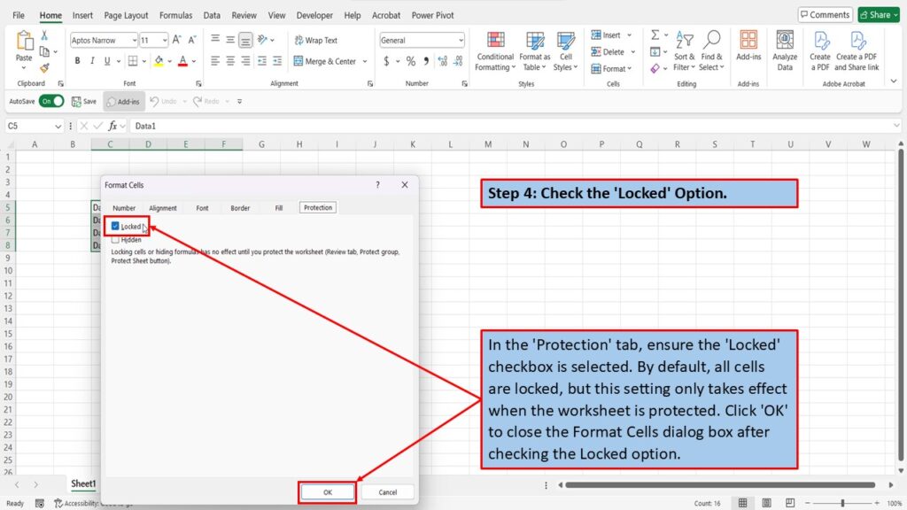
Step 4: Check the ‘Locked’ Option.
By default, the ‘Locked’ checkbox is selected.
If it’s unchecked, click to select it.
Click ‘OK’ to apply the changes and close the dialog box.
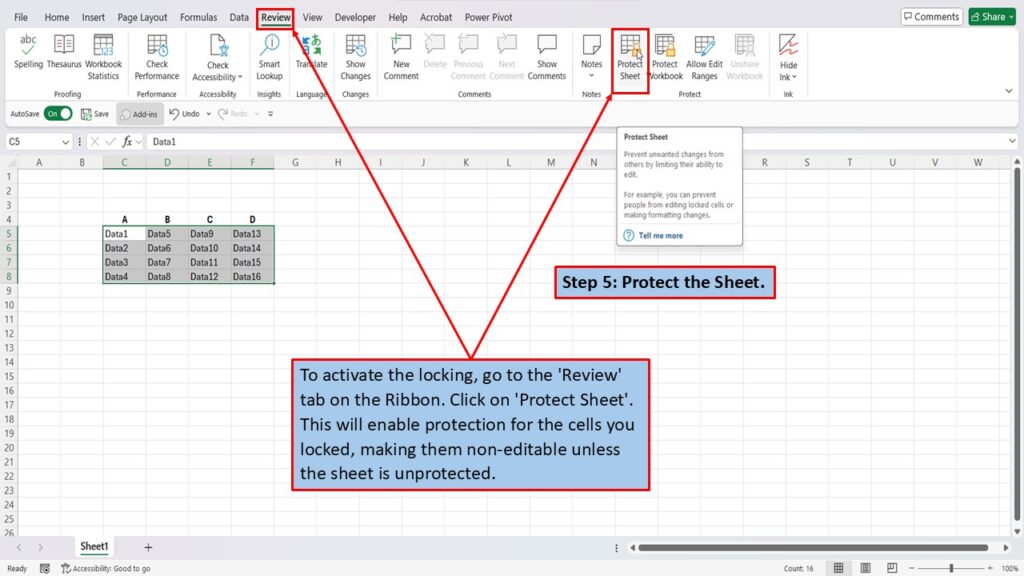
Step 5: Protect the Sheet.
To enforce the locking of the selected cells:
Once you’ve configured your desired settings, click ‘OK’.
Navigate to the Review Tab:
Click on the ‘Review’ tab located on the Excel ribbon.
Initiate Sheet Protection:
Click on ‘Protect Sheet’.
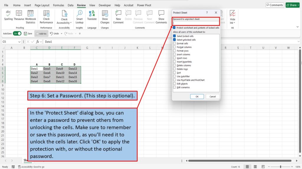
Configure Protection Settings:
A dialog box titled ‘Protect Sheet’ will appear.
Here, you can set a password to prevent others from unprotecting the sheet.
Below the password field, there’s a list of options allowing you to specify what users can do on the protected sheet, such as selecting locked or unlocked cells, formatting cells, inserting rows or columns, etc.
Step 6: Set a Password.
If you entered a password in the previous step, you’ll be prompted to confirm it by re-entering it.
Ensure you remember this password, as you’ll need it to unprotect the sheet in the future.
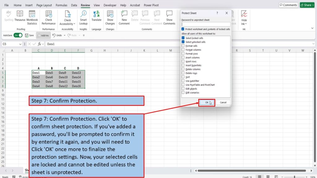
Step 7: Confirm Protection.
Click ‘OK’ to confirm sheet protection. If you’ve added a password, you’ll be prompted to confirm it by entering it again, and you will need to Click ‘OK’ once more to finalize the protection settings. Now, your selected cells are locked and cannot be edited unless the sheet is unprotected.
Additional Considerations:
- Unlocking Specific Cells While Protecting the Rest of the Worksheet:
- If you want most of the worksheet to be protected but allow editing in specific cells:
- Select the entire worksheet by pressing Ctrl + A.
- Open the Format Cells dialog box (Ctrl + 1), navigate to the Protection tab, and uncheck the ‘Locked’ option.
- Click ‘OK’.
- Now, select the cells you want to lock, open the Format Cells dialog box again, and check the ‘Locked’ option.
- Protect the sheet as described in Step 5.
- This approach ensures that only the specified cells are locked, while the rest remain editable.
- If you want most of the worksheet to be protected but allow editing in specific cells:
- Hiding Formulas:
- If you have formulas that you don’t want users to view:
- Select the cells containing the formulas.
- Open the Format Cells dialog box, navigate to the Protection tab, and check the ‘Hidden’ option.
- Protect the sheet.
- Now, when users select these cells, the formula bar will be empty, concealing the formulas.
- If you have formulas that you don’t want users to view:
- Unprotecting the Worksheet:
- To make changes to locked cells or modify protection settings:
- Navigate to the ‘Review’ tab.
- Click on ‘Unprotect Sheet’.
- If a password was set, you’ll be prompted to enter it.
- To make changes to locked cells or modify protection settings:
By following these steps, you can effectively control which parts of your Excel worksheet are editable, ensuring data integrity and preventing accidental or unauthorized changes.
Need More Help?
Video Tutorial
PDF Download