
Hello, and welcome to Mark’s Excel Tips. In this article, I will show you the tenth tip, in a series of 10, tips for Excel charts.
After going through these ten charting tips, you’ll be faster and more efficient than ever before. You can find the links to each of these 10 Excel tips at the bottom of this article. Let’s get started.
Click here to view our video tutorial.
Click here to download our PDF tutorial.
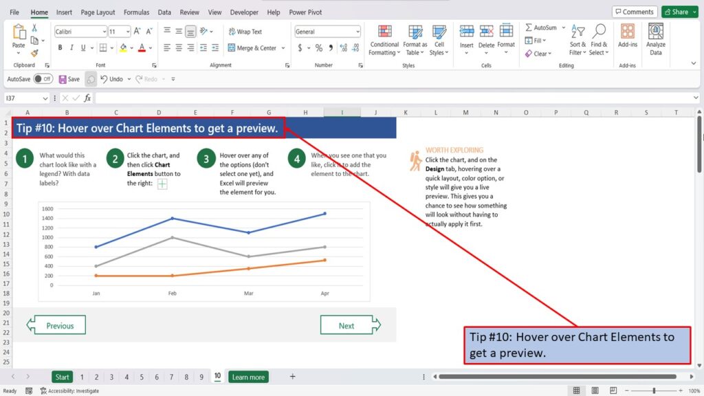
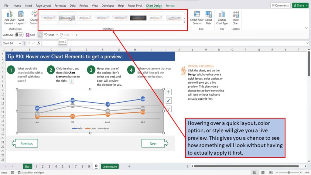
Tip #10: Hover over Chart Elements to get a preview.
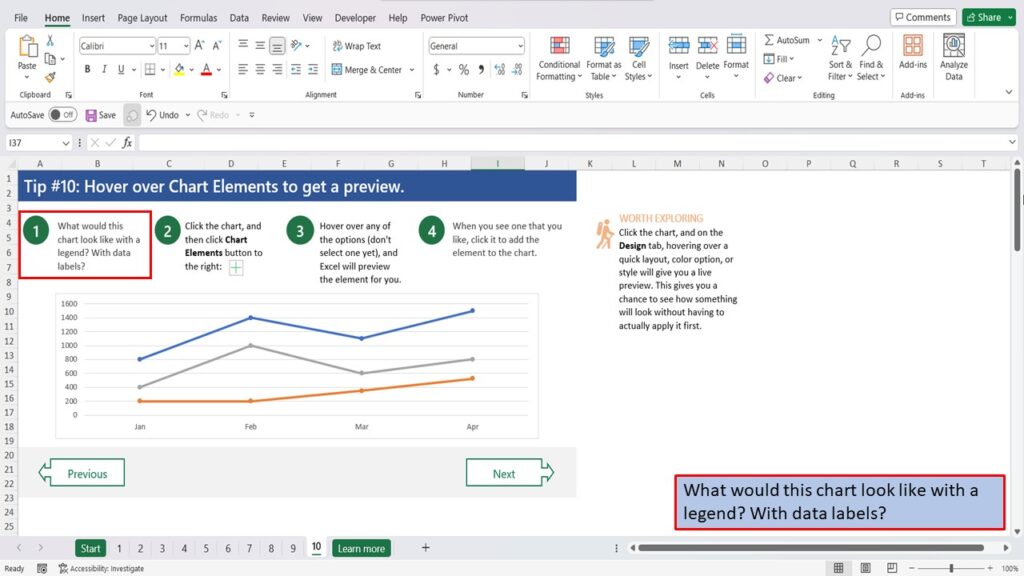
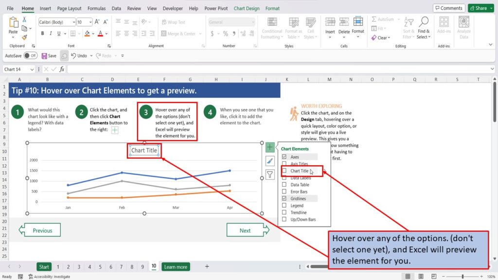
What would this chart look like with a legend? With data labels?
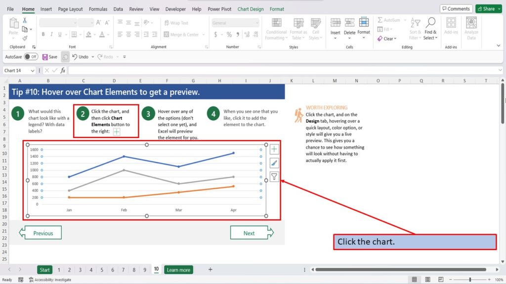
Let’s click on the chart.
And then, click the Chart Elements button to the right.
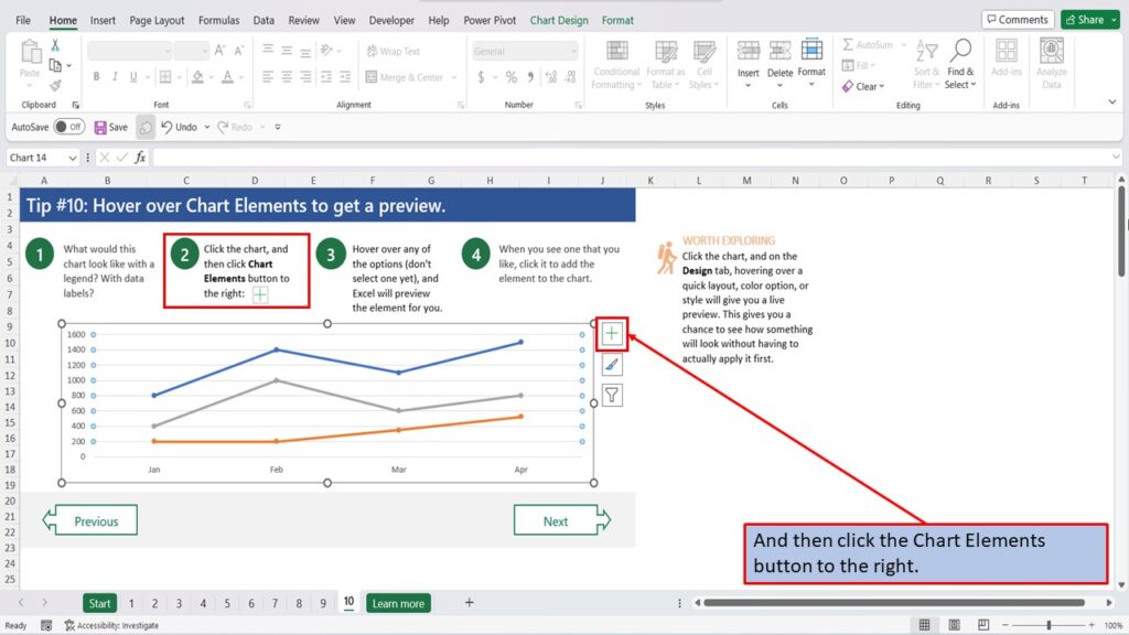
Hover over any of the options. (don’t select one yet), and Excel will preview the element for you.
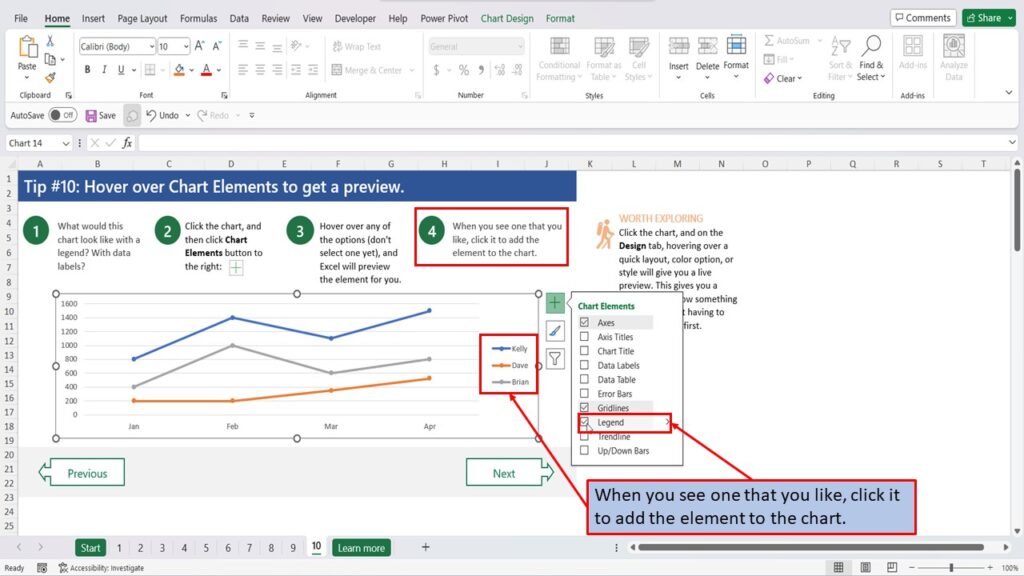
When you see one that you like, click it to add the element to the chart.
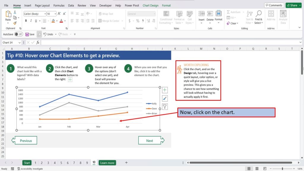
Now click on the chart.
And then, click on the design tab.
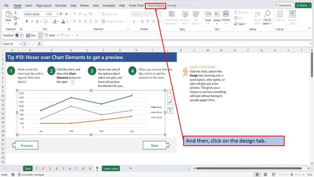
Hovering over a quick layout, color option, or style will give you a live preview. This gives you a chance to see how something will look without having to actually apply it first.
Need More Help?
View the Video Tutorial.
Download this tutorial in PDF by clicking the Download link below.
Tip # 1 | Press Alt + F1 to quickly make a chart
Tip # 2 | Select specific columns, before creating a chart
Tip # 3 | Use a table with a chart
Tip # 4 | Quickly filter data from a chart
Tip # 5 | Use Pivot Charts when your data isn’t summarized
Tip # 6 | Create multi-level labels
Tip # 7 | Use a secondary axis to create a combo chart
Tip # 8 | Hook up a chart title to a cell