Hello, and welcome to Mark’s Excel Tips. In today’s video, we are going to show you how to lock, specific cells in Excel. Let’s get started.
Click here to view our video tutorial.
Click here to download our PDF tutorial.
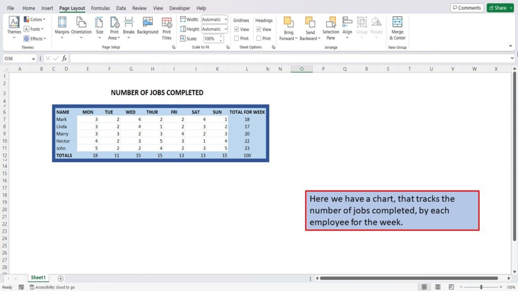
Here we have a chart, that tracks the number of jobs completed, by each employee for the week.
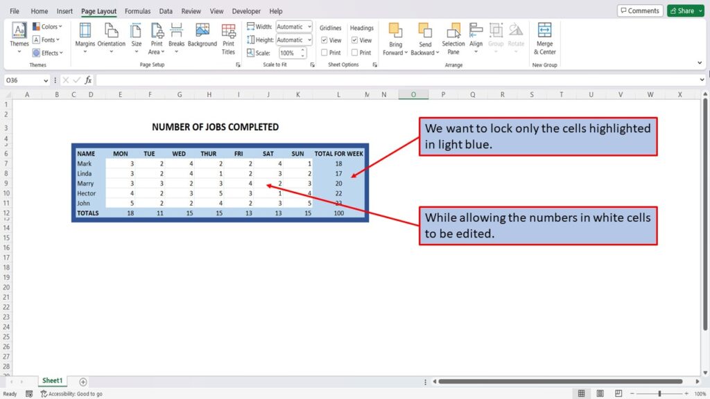
We want to lock only the cells highlighted in light blue. While allowing the numbers in white cells to be edited.
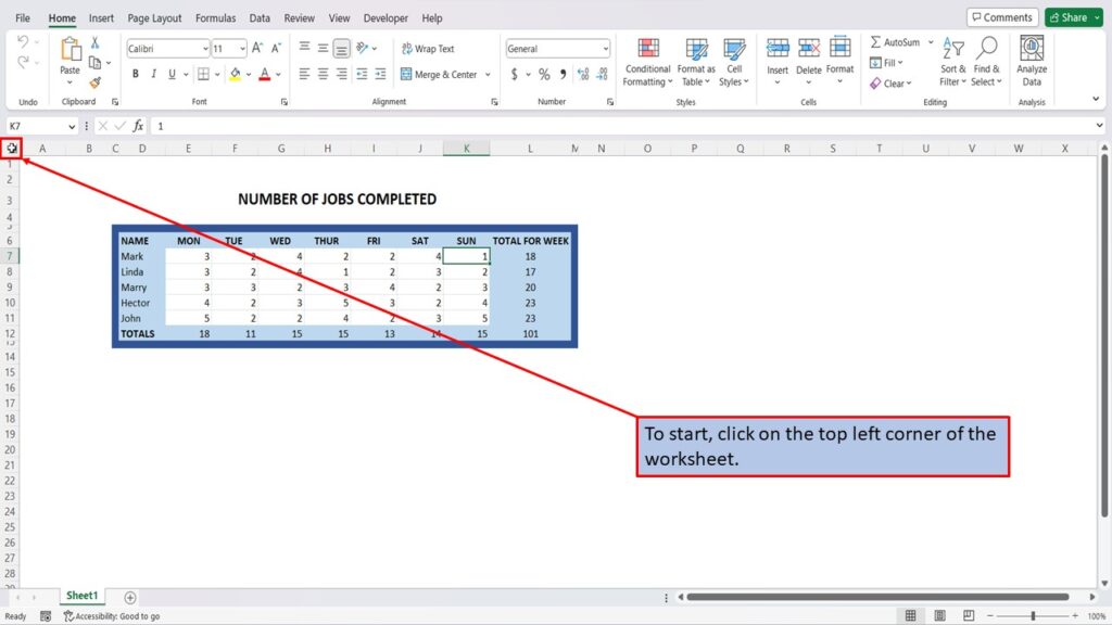
To start, click on the top left corner of the worksheet.
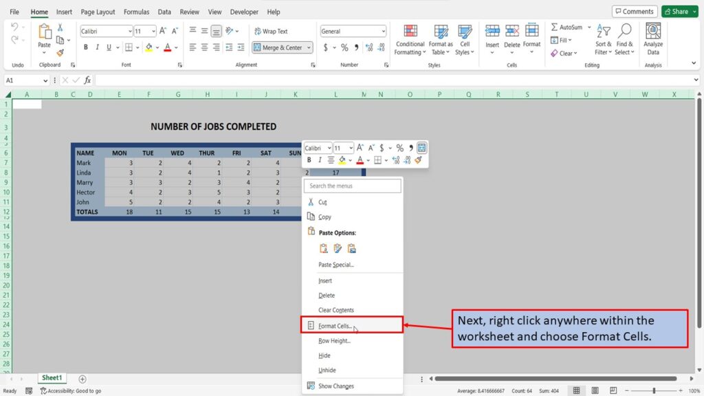
Next, right click anywhere within the worksheet and choose Format Cells.
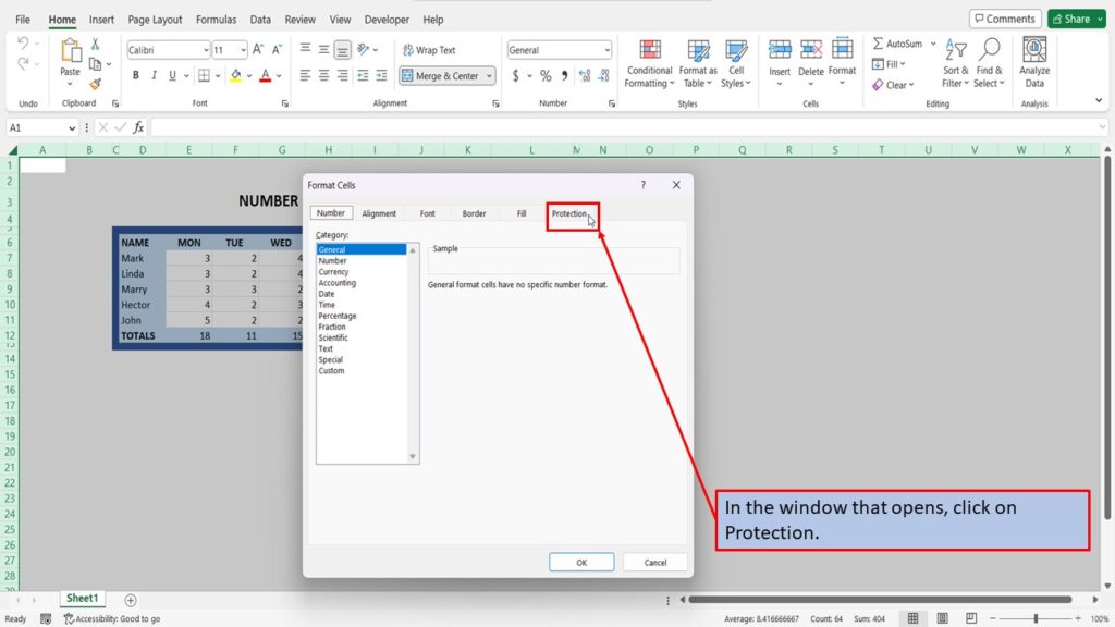
In the window that opens, click on Protection.
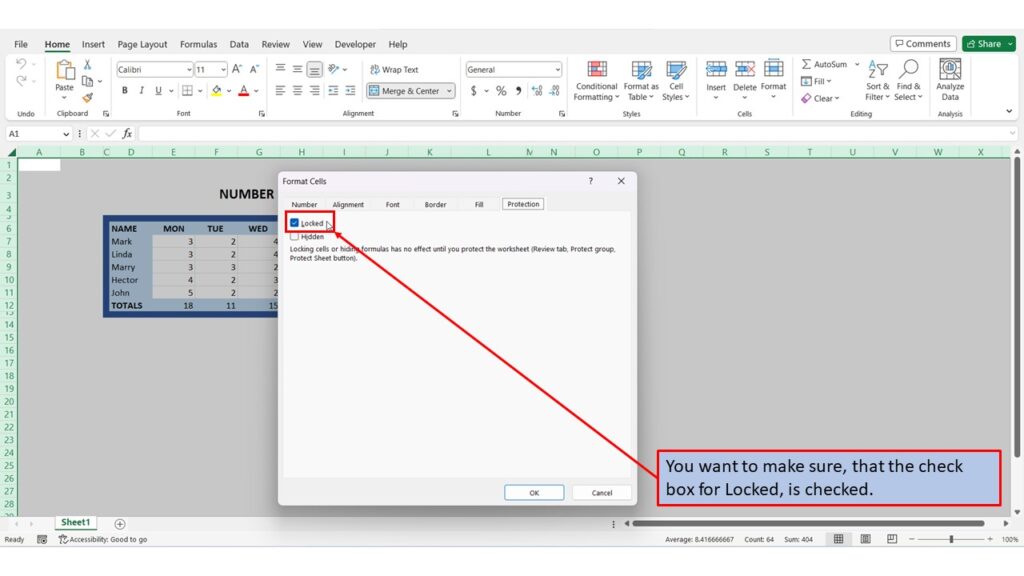
You want to make sure, that the check box for Locked, is checked.
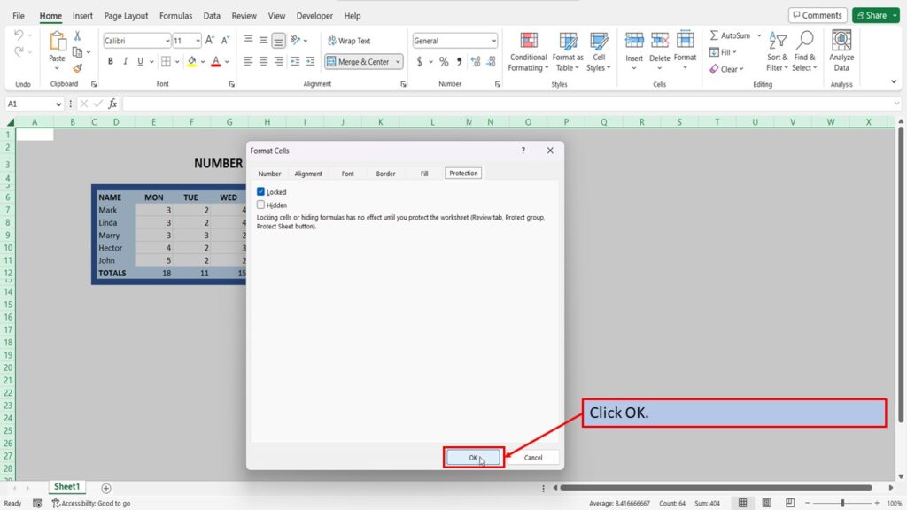
Click OK.
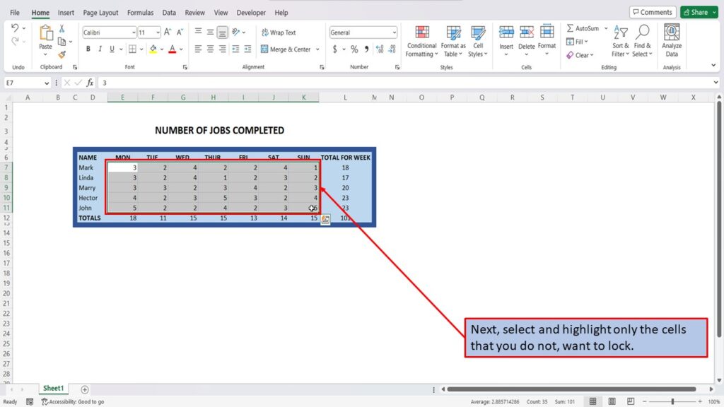
Next, select and highlight only the cells that you do not, want to lock.
Right click within the highlighted area, and choose, Format Cells.
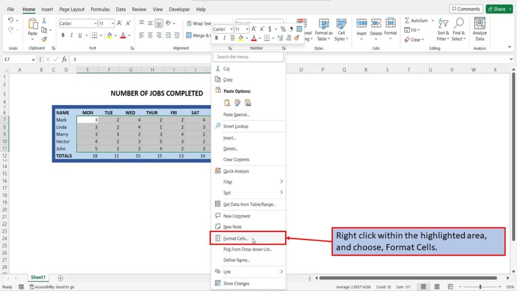
This time, you want to uncheck, the locked checkbox.
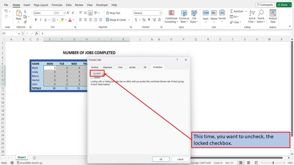
Click OK.
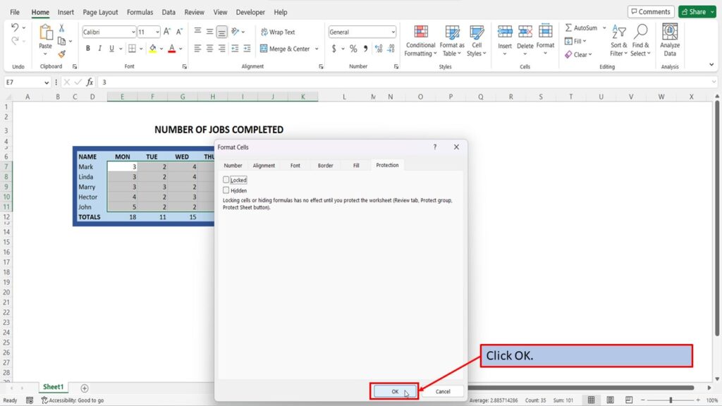
Now, we have just one more step to perform. Click on Review.
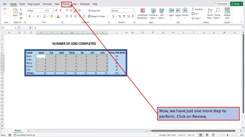
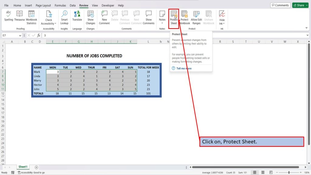
Click on, Protect Sheet.
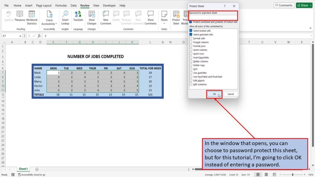
In the window that opens, you can choose to password protect this sheet, but for this tutorial, I’m going to click OK instead of entering a password.
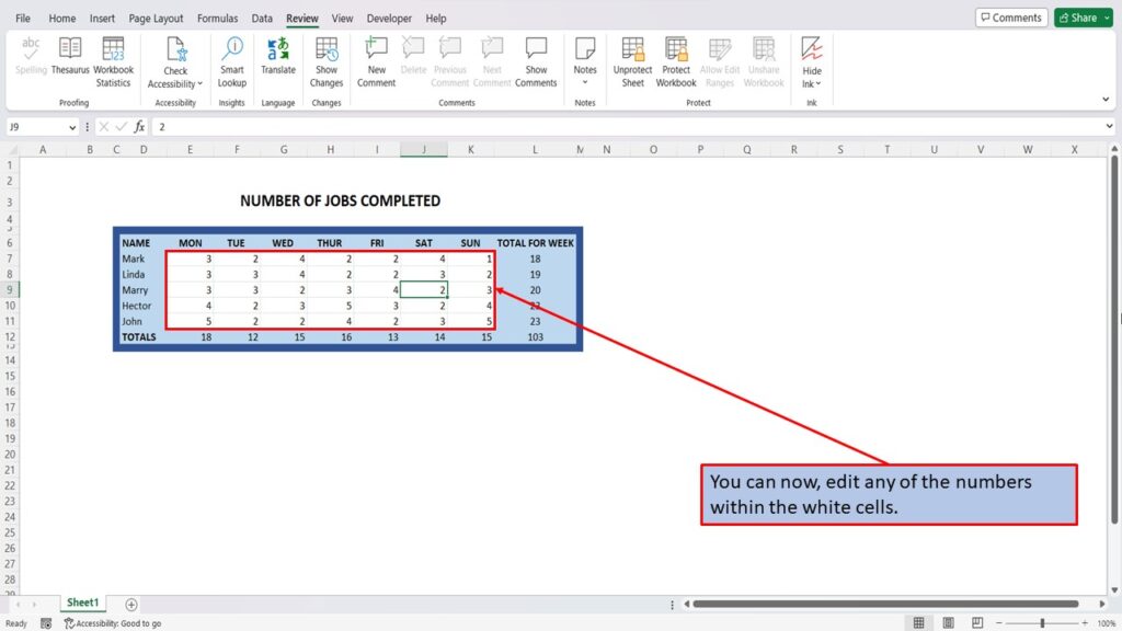
You can now, edit any of the numbers within the white cells.
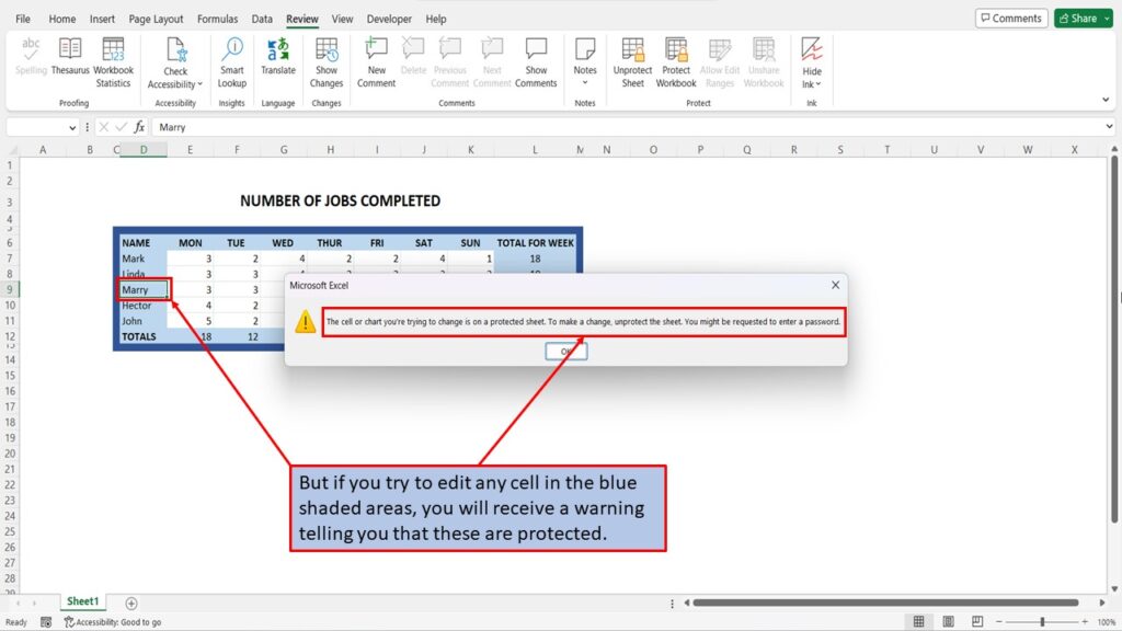
But if you try to edit any cell in the blue shaded areas, you will receive a warning telling you that these are protected.
View the Video Tutorial.
Download this tutorial in PDF by clicking the Download link below.
