Hello, and welcome to Mark’s Excel Tips. Today, we are going to show you how to apply color, to alternate rows using in Excel 365 using format as table. Let’s get started.
You first need to decide which rows that you want to have the alternating colors in, and highlight them.
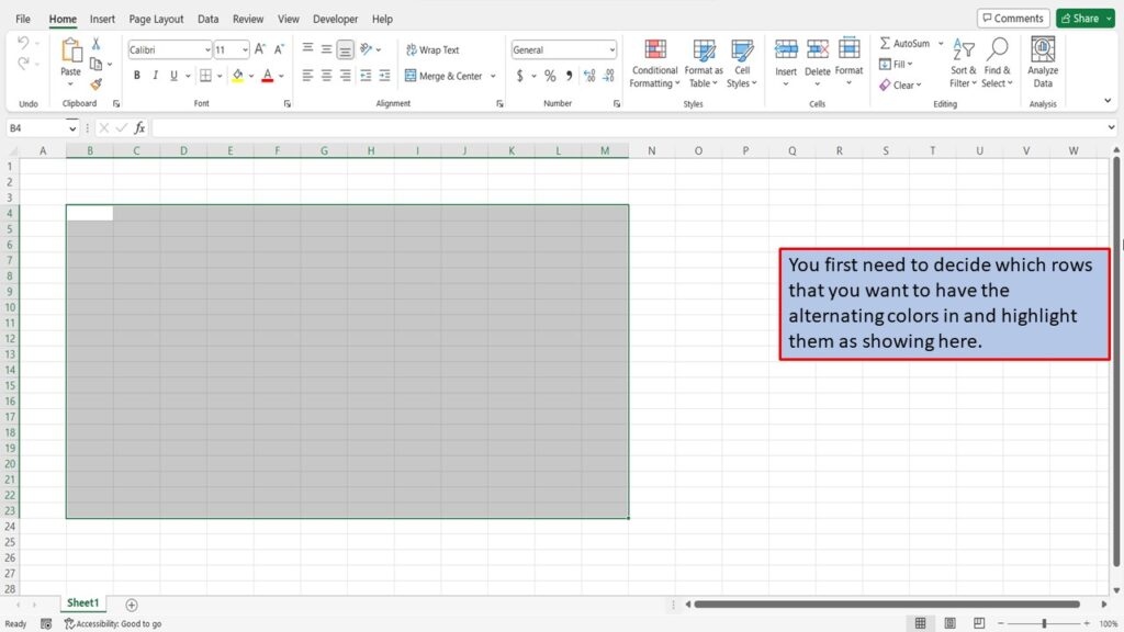
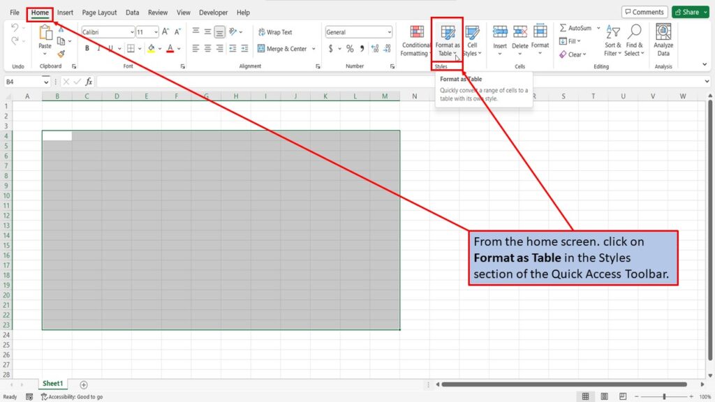
From the home screen. click on Format as Table in the Styles section of the Quick Access Toolbar.
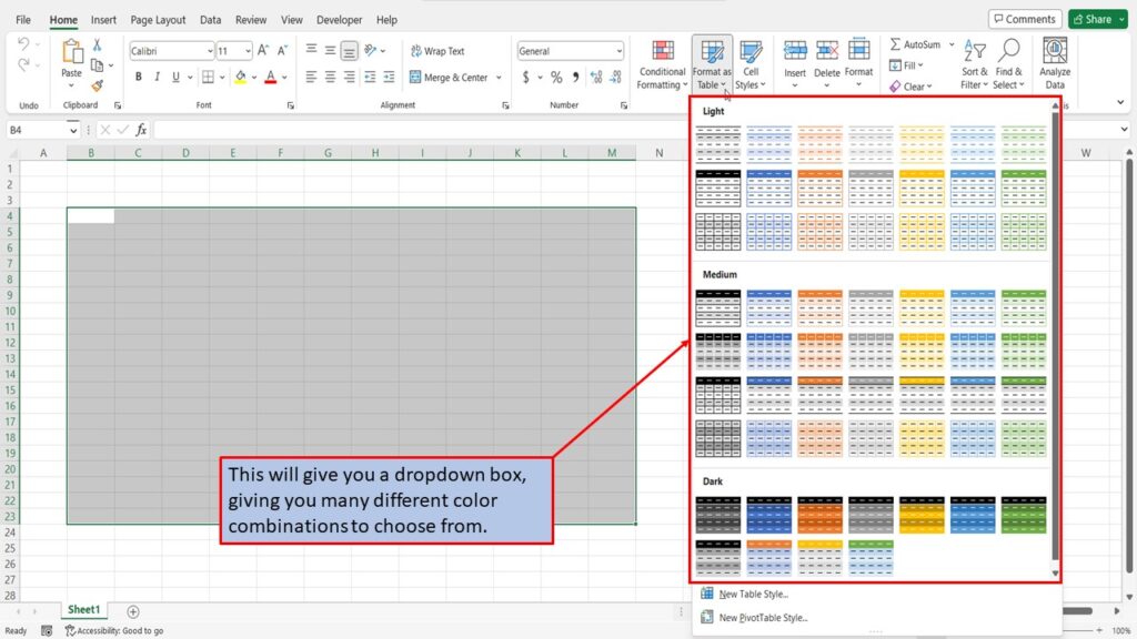
This will give you a dropdown box, giving you many different color combinations to choose from.
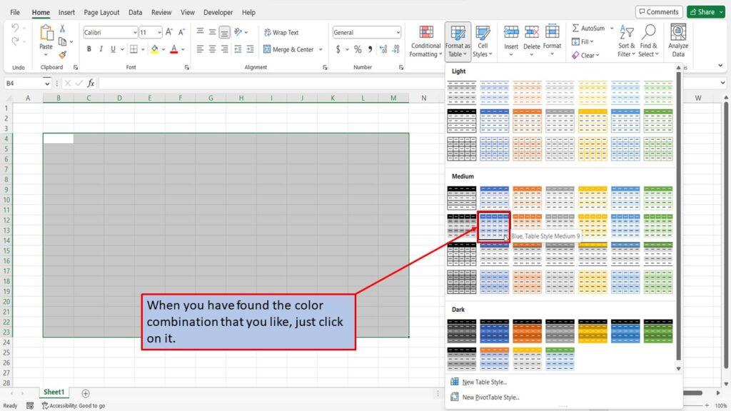
When you have found the color combination that you like, just click on it.
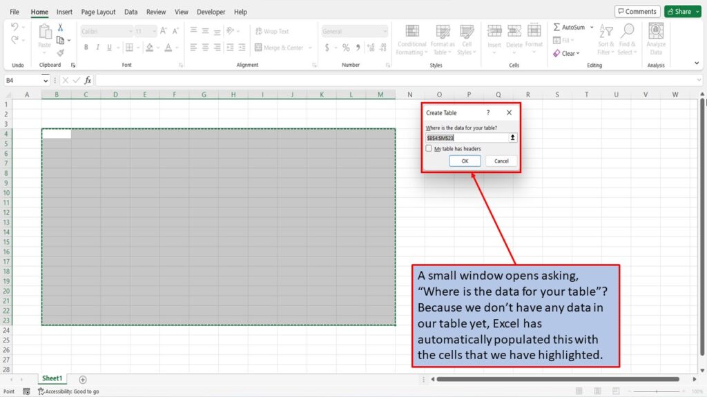
A small window will open asking you, “Where is the data for your table”? Because we don’t have any data in our table yet, Excel has automatically populated this with the cells that we have highlighted.
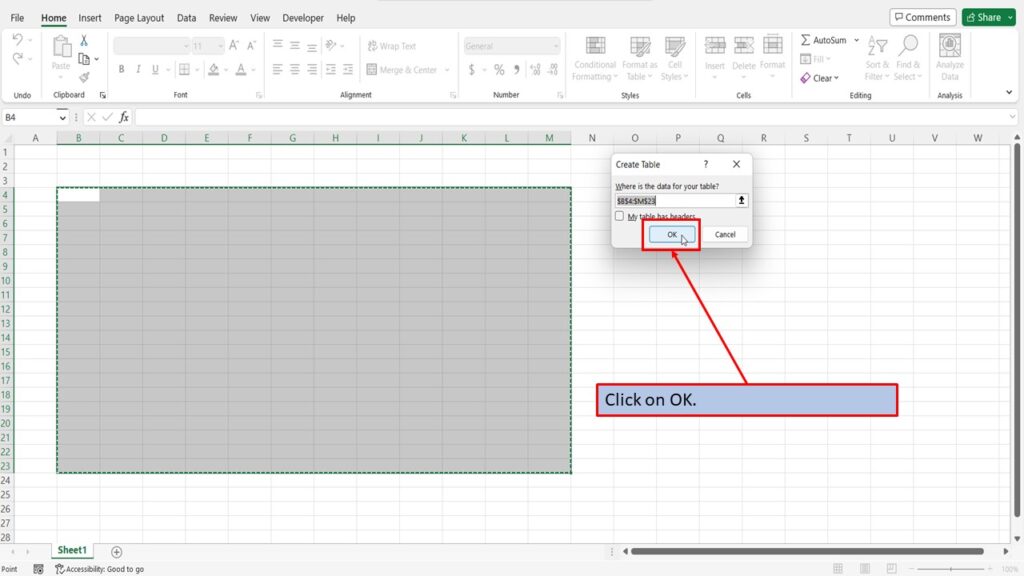
Click on OK.
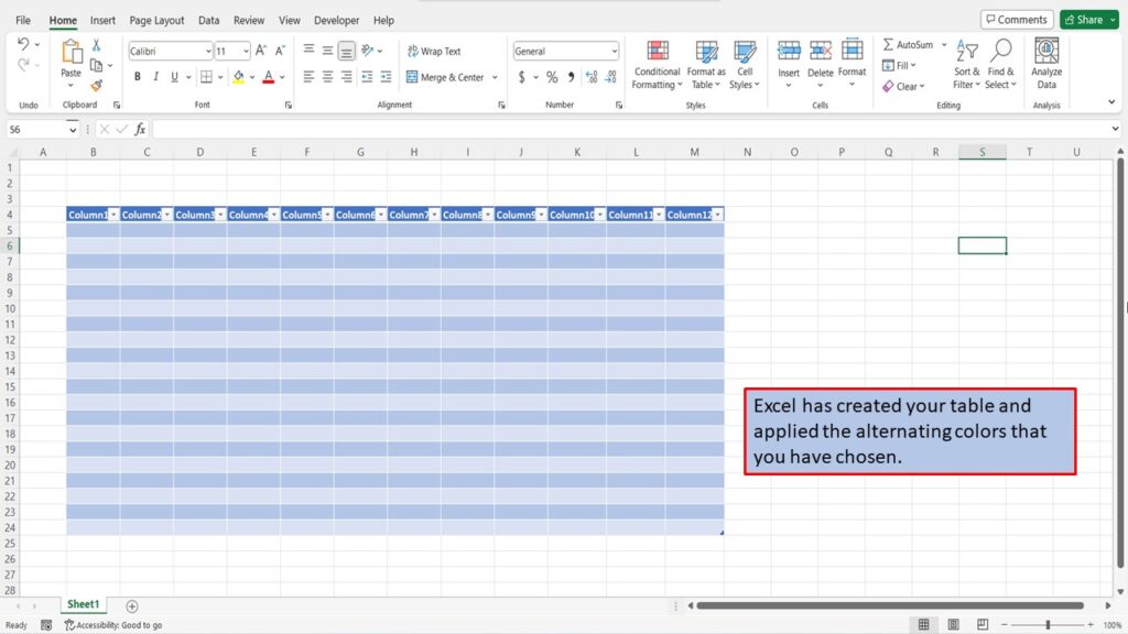
Excel has created your table and applied the alternating colors that you have chosen.
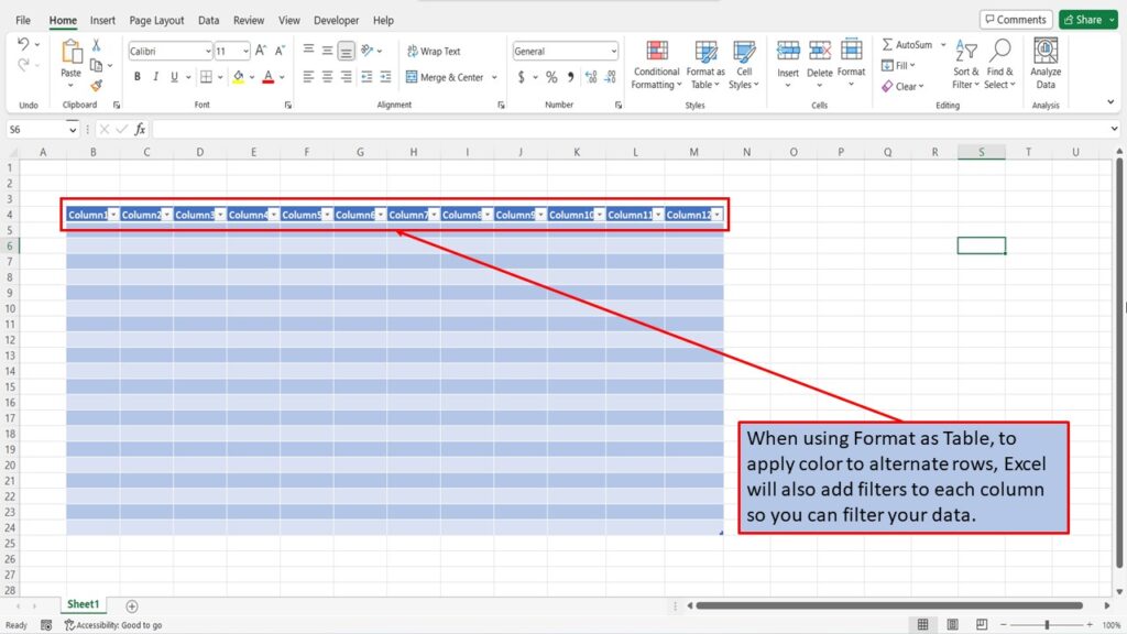
When using Format as Table to apply color to alternate rows, Excel will also add filters to each column so you can filter your data.
Here is a video walking you through each step on how to apply color to alternate rows using formatting in Excel 365.
View the video tutorial below.
You can download this tutorial in PDF format by clicking Download below.
