
Click here to view our video tutorial.
Click here to download our PDF tutorial.
Want to add traffic light icons to your Excel data to quickly spot trends? In this guide, I’ll show you exactly how to use conditional formatting traffic lights in Excel, step by step. Whether you’re tracking task progress, sales goals, or any other data, traffic lights offer an easy way to visualize your results at a glance. Let’s get started!
Understanding Your Data
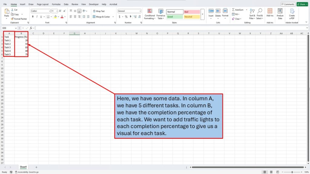
Here, we have some data. In column A, we have 5 different tasks. In column B, we have the completion percentage of each task. Our goal is to add traffic light icons to each completion percentage to give us a visual indicator of task progress. This makes it easy to see which tasks are on track, which need attention, and which are falling behind.
Why Use Whole Numbers Instead of Percentages?
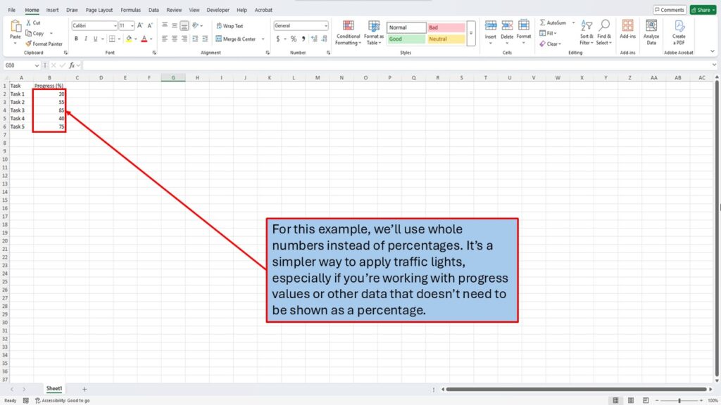
For this example, we’ll use whole numbers instead of percentages. It’s a simpler way to apply traffic lights, especially if you’re working with progress values or other data that doesn’t need to be displayed as a percentage. Using whole numbers also makes it easier to set fixed thresholds for the traffic light colors.
Select Your Data
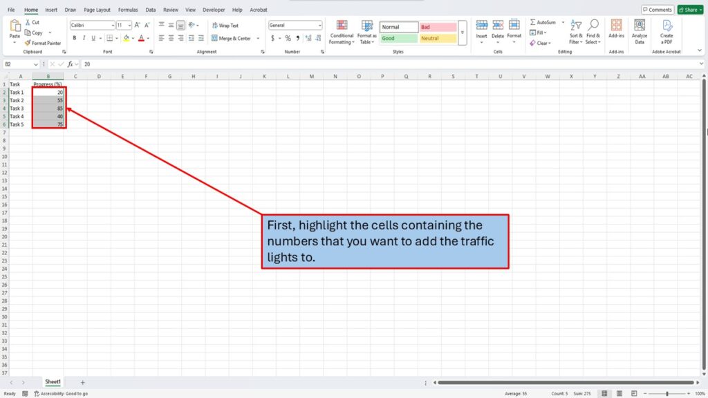
First, highlight the cells containing the numbers that you want to add the traffic lights to. In this example, we’ll select the values in column B, which represent the task completion percentages.
Open Conditional Formatting
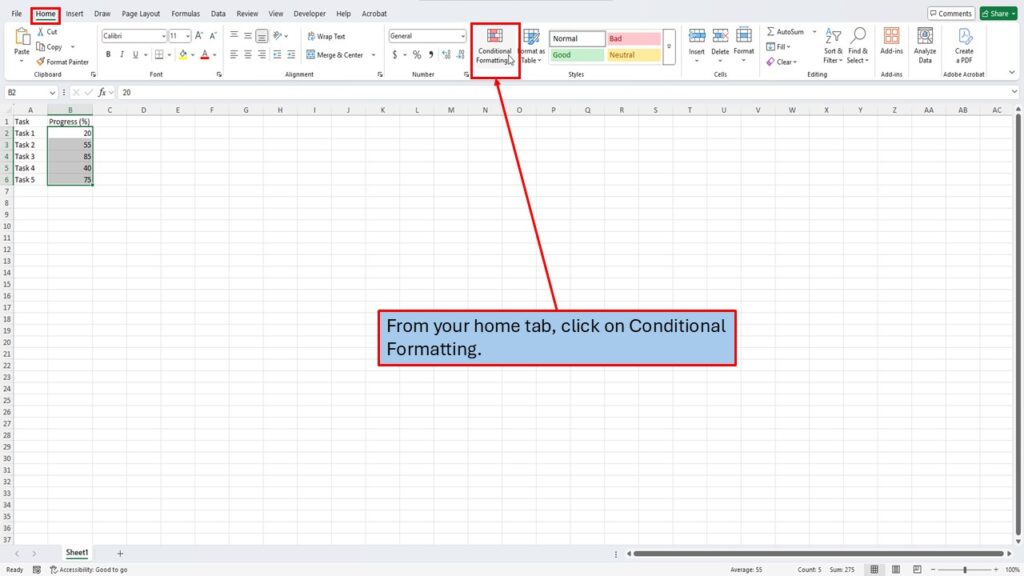
From your Home tab on the Excel ribbon, click on Conditional Formatting. Conditional formatting is a powerful feature in Excel that allows you to apply visual formatting based on the values in your cells.
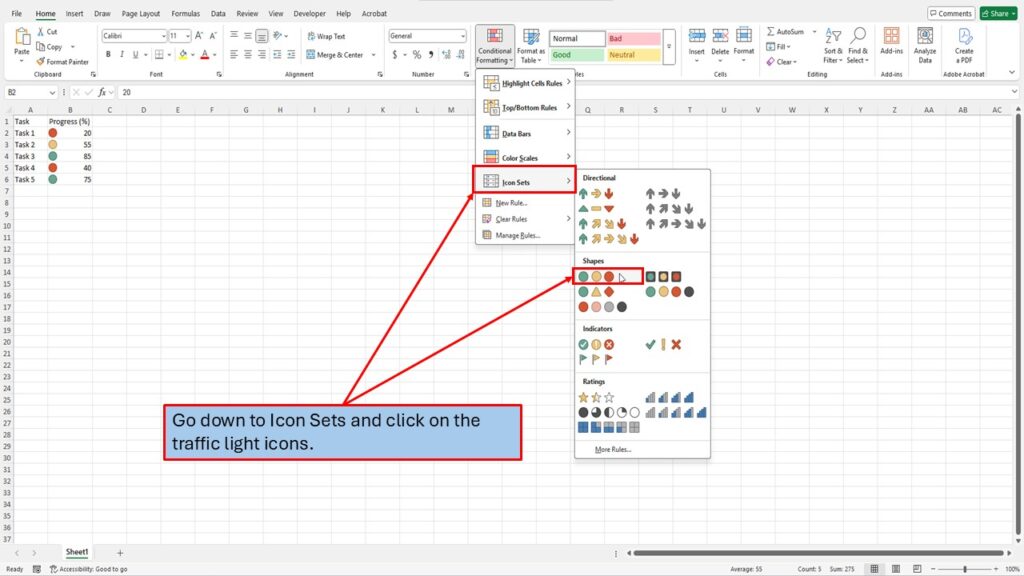
Choose Icon Sets
Next, go down to Icon Sets and select the 3 Traffic Lights (Unrimmed). These are simple, clean traffic light icons that provide a clear visual representation of your data. Excel will apply the default settings for the traffic lights, but we’ll customize them in the next steps.
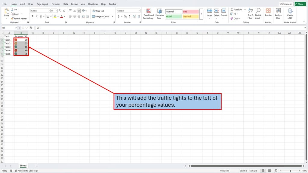
See the Initial Traffic Lights
At this point, Excel will add the traffic lights to the left of your percentage values. However, these are just the default icons. The next step is to customize them to fit your specific needs.
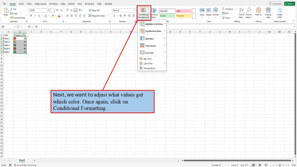
Adjust the Traffic Light Values
To adjust which values display which color, go back to Conditional Formatting.
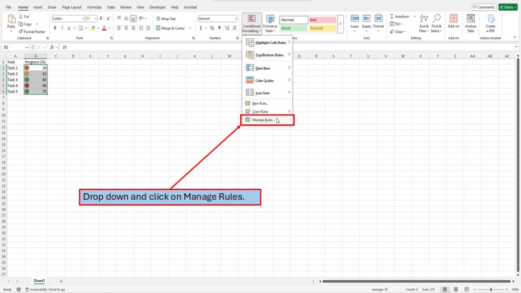
Manage Rules
From the dropdown, click on Manage Rules. This opens the Conditional Formatting Rules Manager, where you can view and edit all the rules applied to your data.
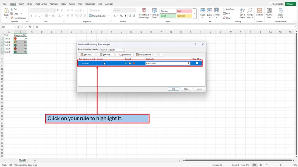
Select the Rule to Edit
Click on the rule that applies the traffic lights to your data. You’ll see it highlighted in the list.
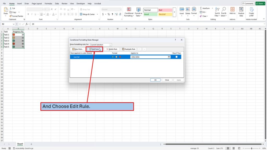
Then, choose Edit Rule to customize it further.
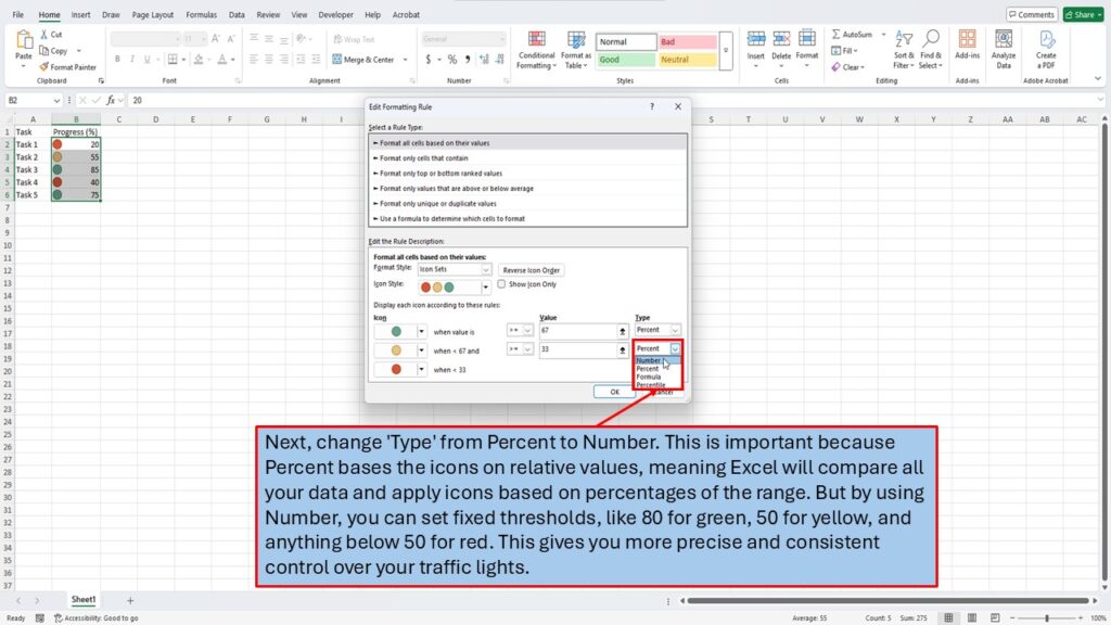
Change Percent to Number
Next, change the ‘Type’ from Percent to Number. This step is important because using Percent bases the icons on relative values. Excel will compare all your data and apply icons based on percentages of the range. By using Number instead, you can set fixed thresholds, like 80 for green, 50 for yellow, and anything below 50 for red. This gives you more precise and consistent control over your traffic lights.
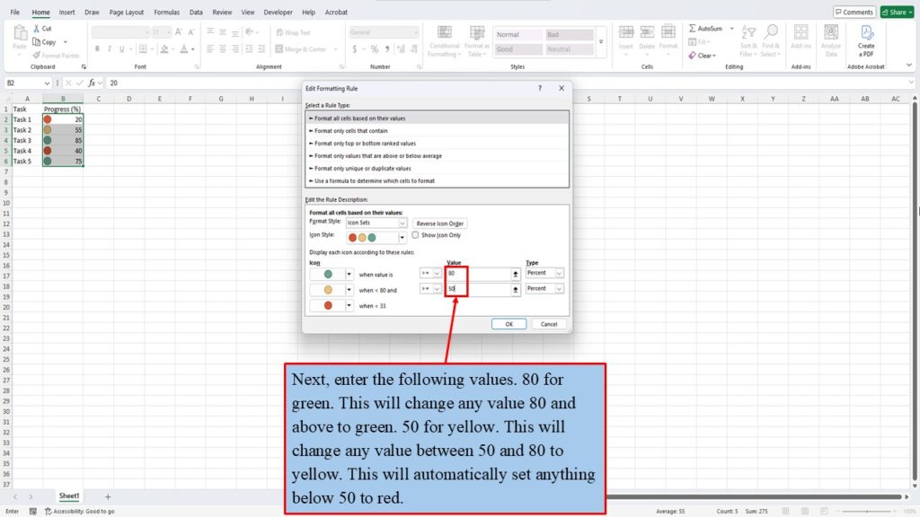
Set Your Values
Now, enter the following values:
- 80 for Green: Any value 80 or above will display a green light.
- 50 for Yellow: Any value between 50 and 80 will show a yellow light.
- Anything below 50 will automatically be marked with a red light.
- These thresholds will give you a clear visual overview of your data.
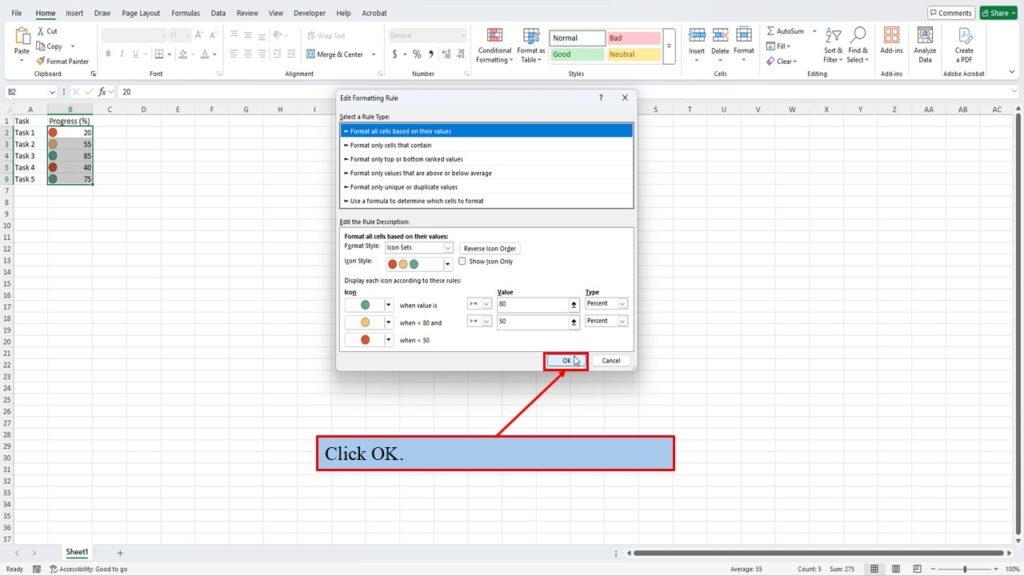
Apply the Changes
Click OK to save your rule settings.
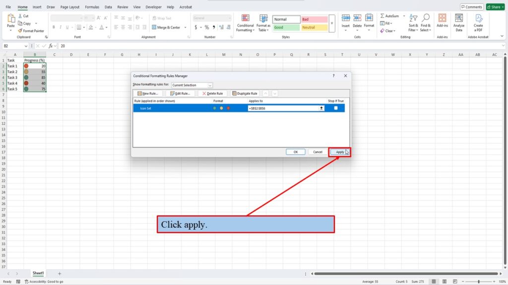
Apply the Formatting
Click Apply in the Conditional Formatting Rules Manager to see your traffic lights update in real-time.
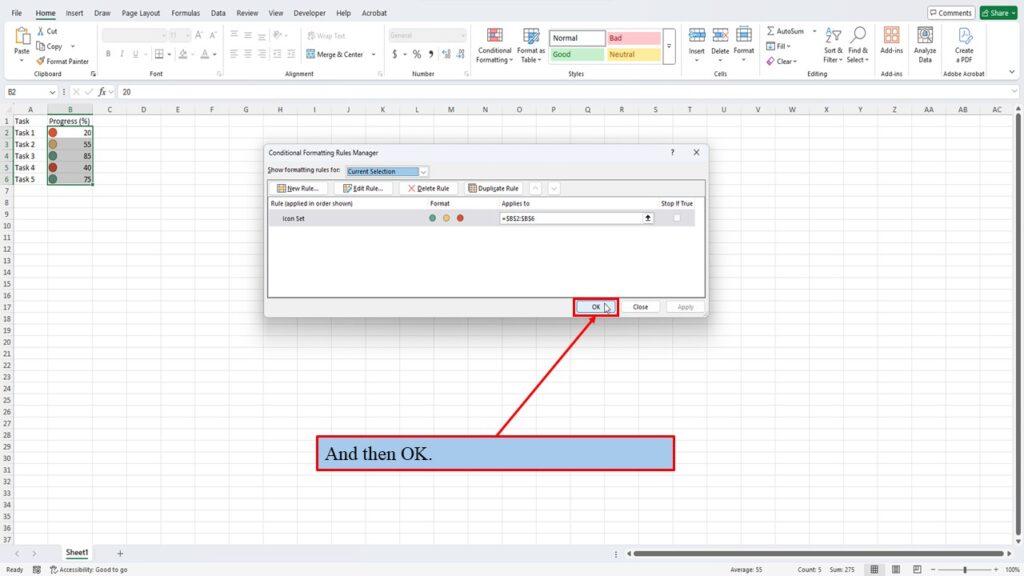
Confirm and Finish
Finally, click OK one more time to close the Rules Manager. Your traffic lights should now be applied, giving you an easy way to analyze your data at a glance.
Conclusion
And that’s it! You now know how to use conditional formatting traffic lights in Excel using whole numbers. It’s a quick and effective way to add visual insights to your data.
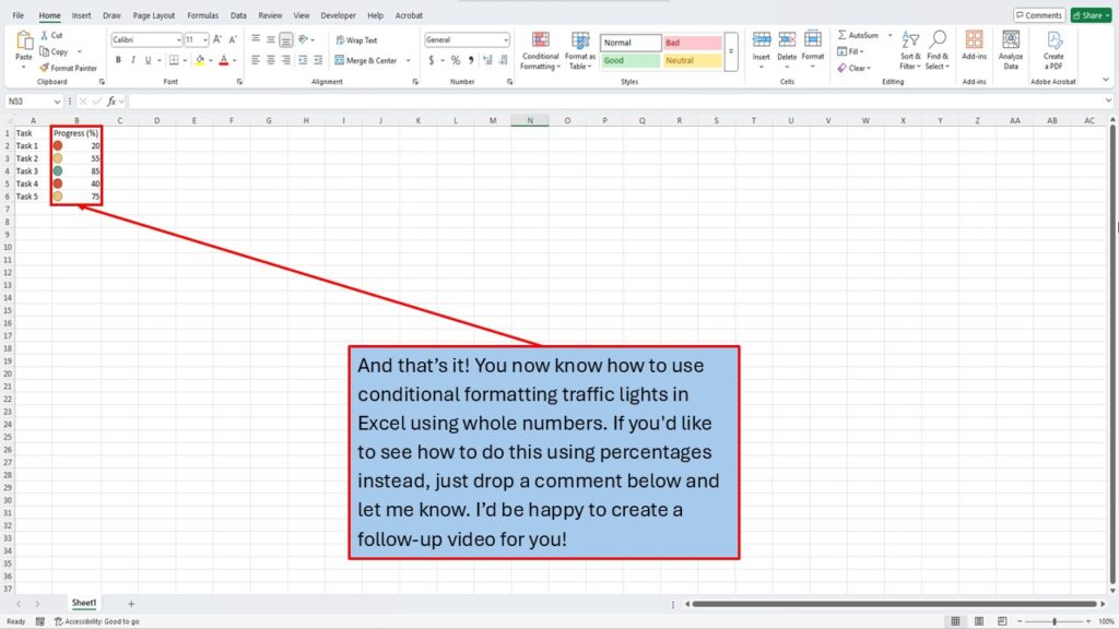
If you’d like to see how to do this using percentages instead, just drop a comment below and let me know. I’d be happy to create a follow-up video or post for you!
For more Excel tips and tutorials, be sure to check out my other guides. And if you found this helpful, feel free to share it with others who might benefit!
Need More Help?
Video Tutorial
Download The PDF Below
You might also like: Master Excel Navigation: Alt Key Shortcuts Made Simple!
Visit My YouTube Channel