
Click here to view our video tutorial.
Click here to download our PDF tutorial.

These step by step instructions will show you exactly how to use AutoSum in Excel, using only shortcut keys. No mouse needed! In this quick and clear demonstration, I’ll walk you step-by-step through adding up columns and rows using only your keyboard. Whether you have difficulty using a mouse, prefer shortcut keys, or simply want a faster workflow, this tutorial has you covered. Let’s jump right in!
Step 1:
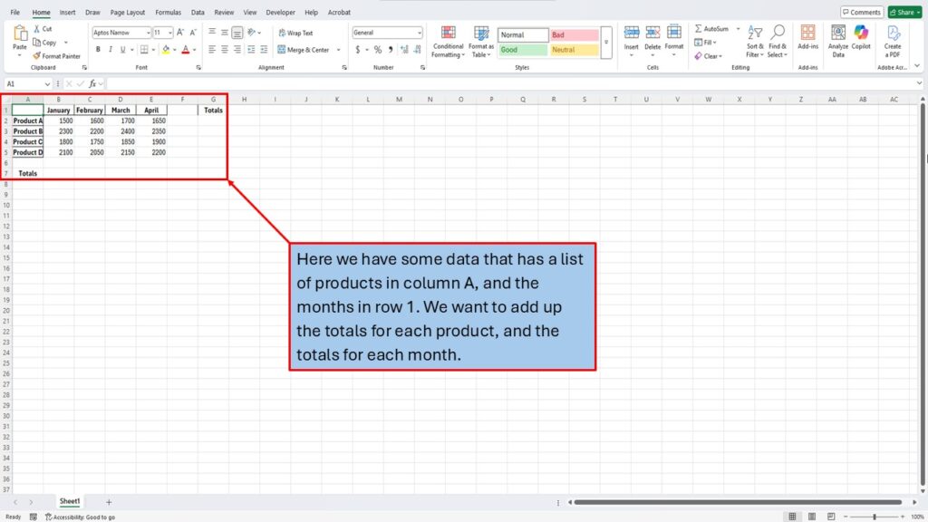
Here we have a simple sales data spreadsheet in Excel, listing different products in column A and monthly sales figures in row 1. Our goal is to quickly calculate the totals for each product (rows) and each month (columns) using Excel’s powerful AutoSum feature, entirely through keyboard shortcuts—no mouse clicks necessary!
Step 2:
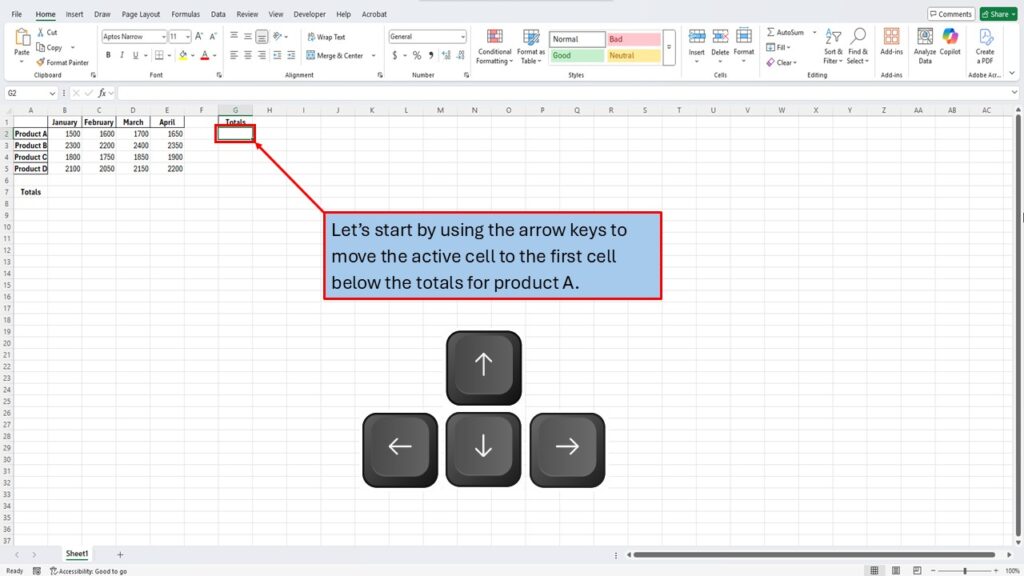
To begin summing up our product totals, we’ll first use the arrow keys on the keyboard to navigate the active cell down to the first empty cell immediately following the data for Product A. In our example, this will be cell G2, where the total for Product A’s monthly sales will appear.
Step 3:
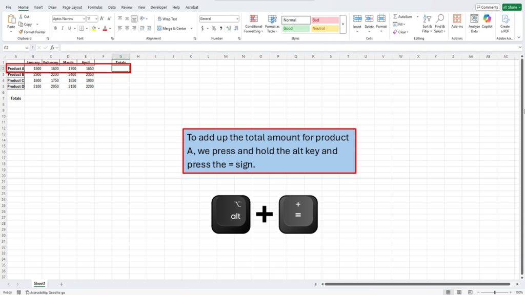
With the active cell (G2) now selected, press and hold the Alt key and then press the equals (=) sign. This shortcut triggers Excel’s AutoSum feature instantly, saving you from having to type out the SUM formula manually.
Step 4:
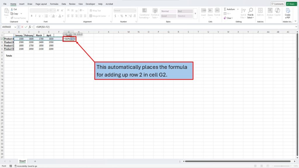
As soon as you use the shortcut, Excel will automatically insert the correct formula, =SUM(B2:F2), directly into cell G2, highlighting the cells being summed for easy visual confirmation.
Step 5:
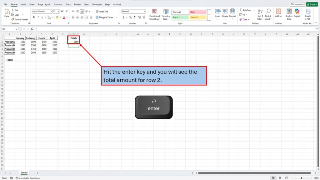
To finalize the calculation, simply press the Enter key. Excel instantly calculates and displays the total monthly sales for Product A right in cell G2.
Step 6:
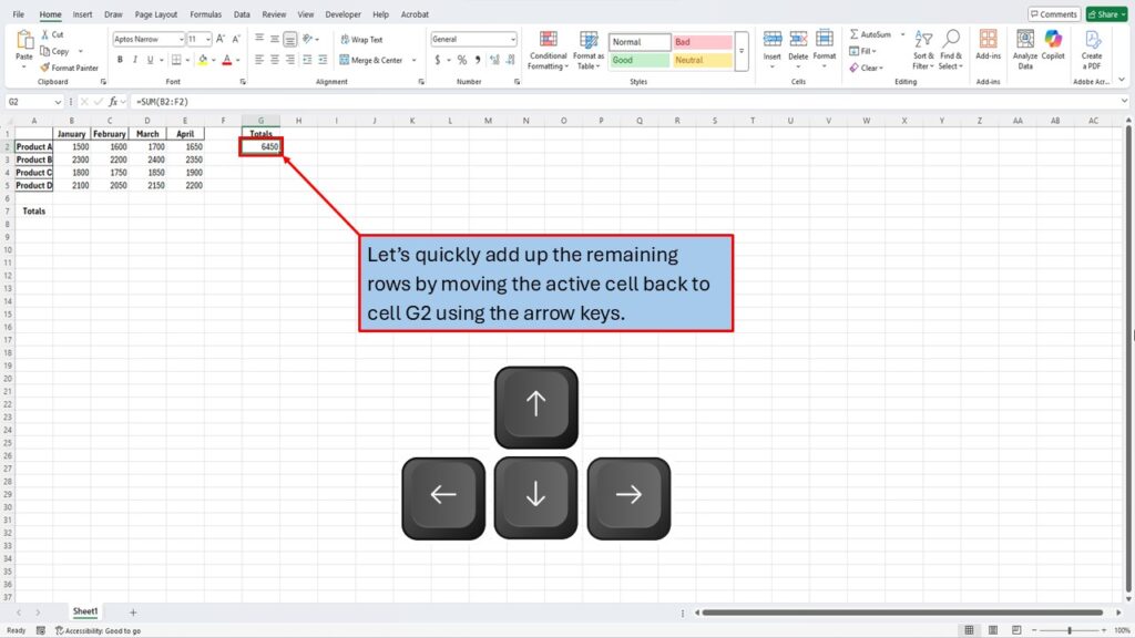
Now let’s rapidly add totals for the remaining products. First, navigate back to cell G2 using the arrow keys. We’re going to copy the formula we’ve already created and quickly paste it down into the cells below.
Step 7:
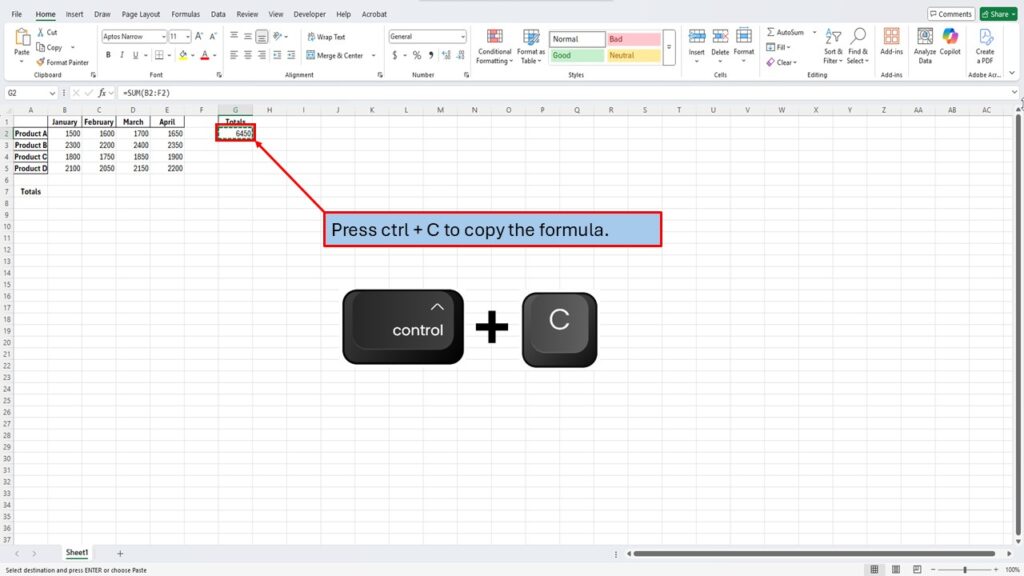
Press the keyboard shortcut Ctrl + C to copy the AutoSum formula from cell G2. You’ll see the cell highlighted to indicate the formula has been copied.
Step 8:
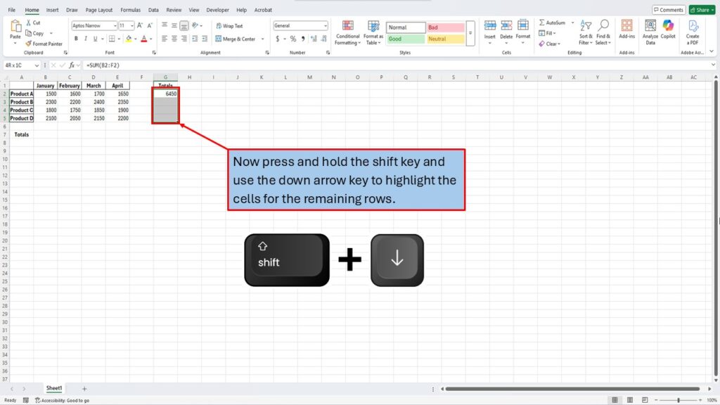
Next, hold down the Shift key, and while keeping it held, use the down arrow key to select (highlight) all cells below (G3 through G5). These are the cells that will display the total sales for Products B through D.
Step 9:
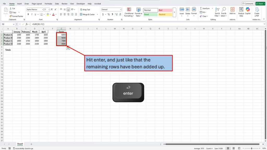
Once the cells are highlighted, press the Enter key again. Excel instantly calculates and displays totals for all remaining products, completing your row totals quickly and effortlessly.
Step 10:
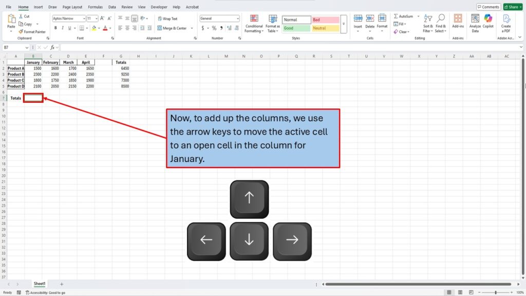
With row totals completed, let’s now calculate the column totals to find the monthly sales sums. Use the arrow keys to move your active cell to the empty cell directly below the data for January, which in our example spreadsheet is cell B7.
Step 11:
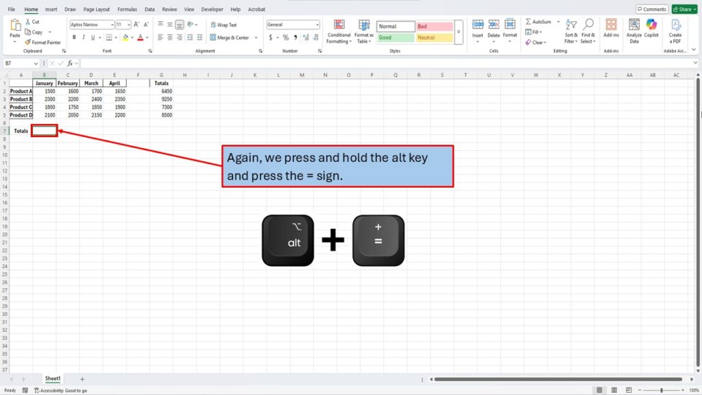
Again, press and hold the Alt key on your keyboard and then press the equals (=) sign to trigger the AutoSum shortcut. This will automatically insert the formula you need to sum the column of numbers above.
Step 12:
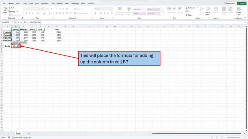
Excel automatically places the correct SUM formula (=SUM(B2:B5)) into cell B7, clearly indicating which cells it will total. You can verify visually that the correct column of numbers has been selected.
Step 13:
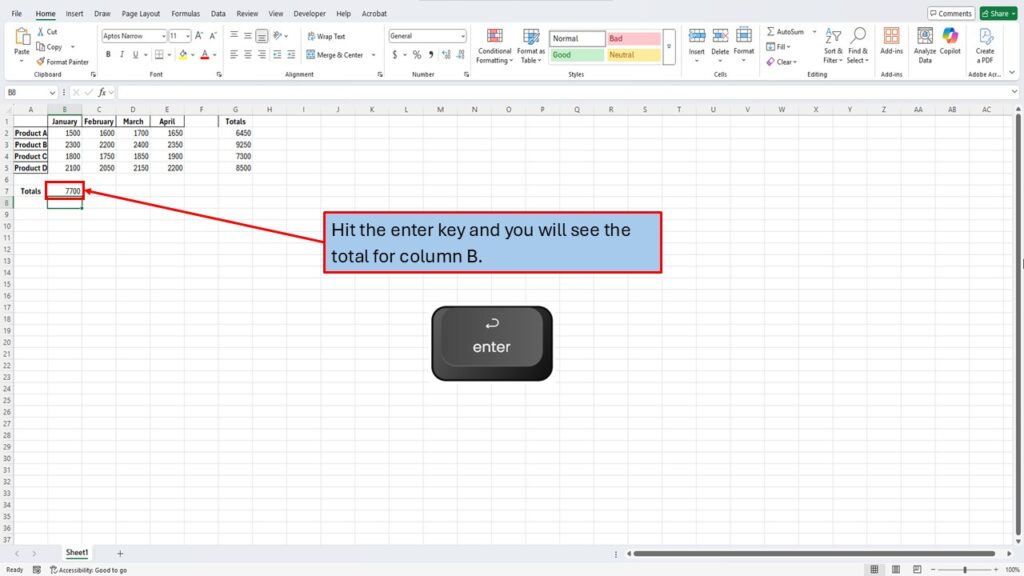
Hit the Enter key, and Excel calculates and displays the total sales for January right in cell B7, providing immediate insight into the monthly total.
Step 14:
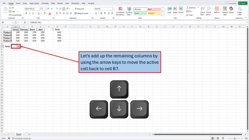
To finish calculating totals for the remaining months, move the active cell back to cell B7 with your arrow keys. We’re going to use the copy-and-paste shortcut method again to rapidly populate the remaining totals.
Step 15:
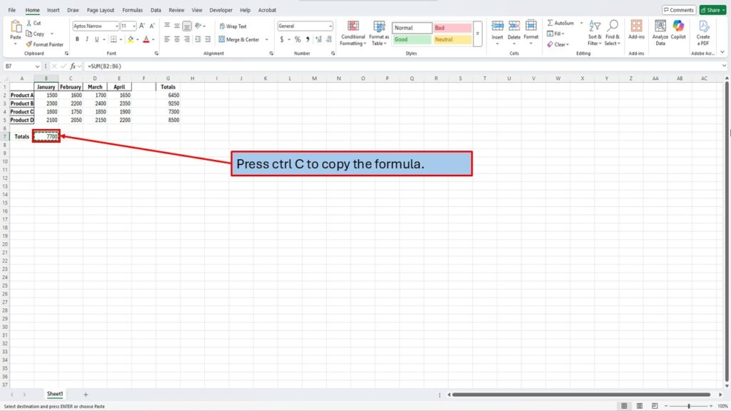
Press Ctrl + C to copy the formula from cell B7. This prepares Excel to replicate the formula for each subsequent month.
Step 16:
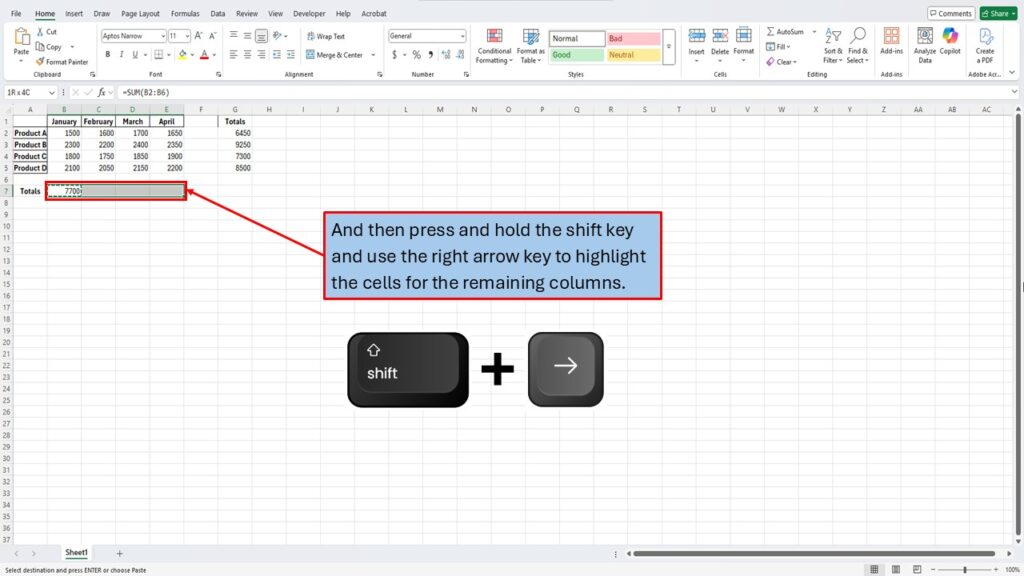
Now, hold down the Shift key and use the right arrow key to select (highlight) the remaining empty cells (C7 through F7) for February, March, and April totals.
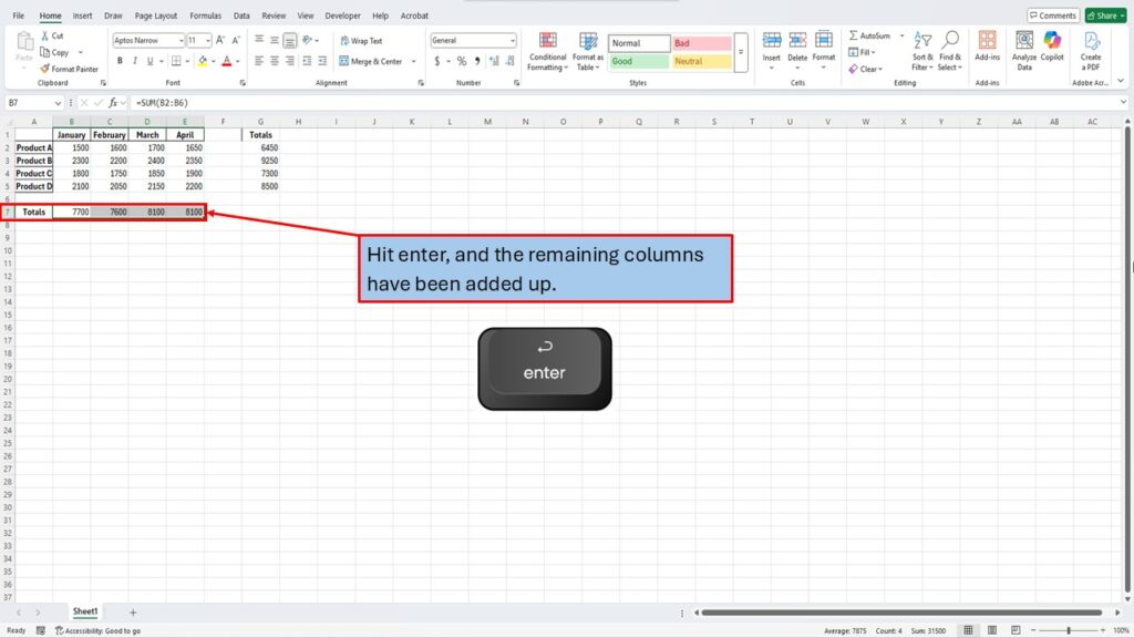
Step 17:
Finally, press the Enter key one more time. Excel instantly calculates and displays the totals for all remaining months, completing the process of summing both rows and columns entirely using shortcut keys.
Need More Help?
Video Tutorial
Download PDF Below
You May Also Like: Quickly Hide Columns With Keyboard Shortcuts in 2025
Visit My YouTube Channel