
Click here to view our video tutorial.
Click here to download our PDF tutorial.
Want to hide and unhide rows and columns in Excel using only shortcut keys? In this video, I’ll show you exactly how to do it. quickly and efficiently! No mouse needed, just your keyboard. We’ll cover four simple steps. hiding rows, hiding columns, unhiding rows, and unhiding columns. I will also show you what to do if any of these steps should fail to unhide your rows and columns. Let’s get started!
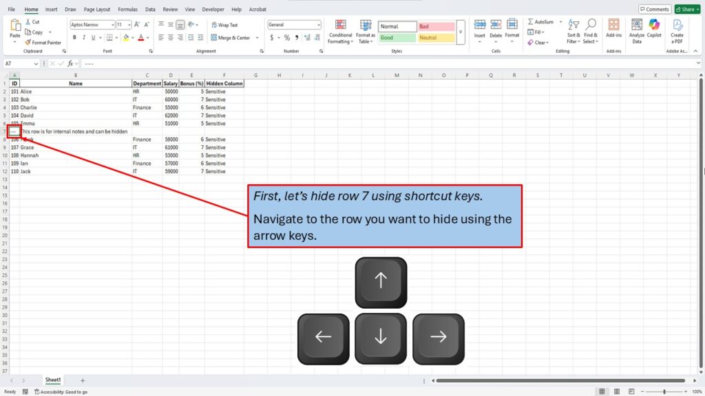
- Identify the Row to Hide:
Begin by determining which row you want to hide. For instance, if you aim to hide row 7, use the arrow keys to navigate to any cell within that row.
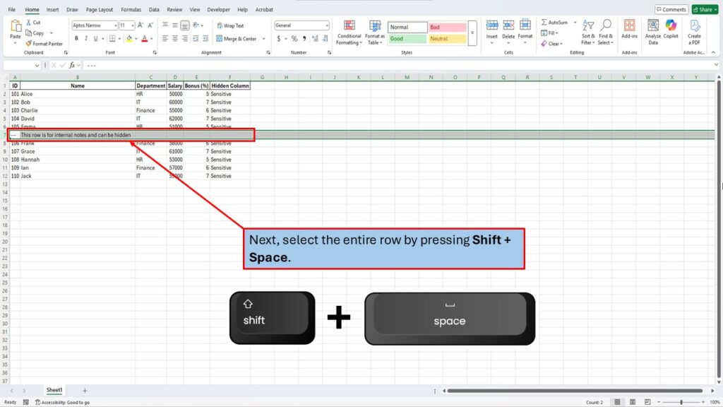
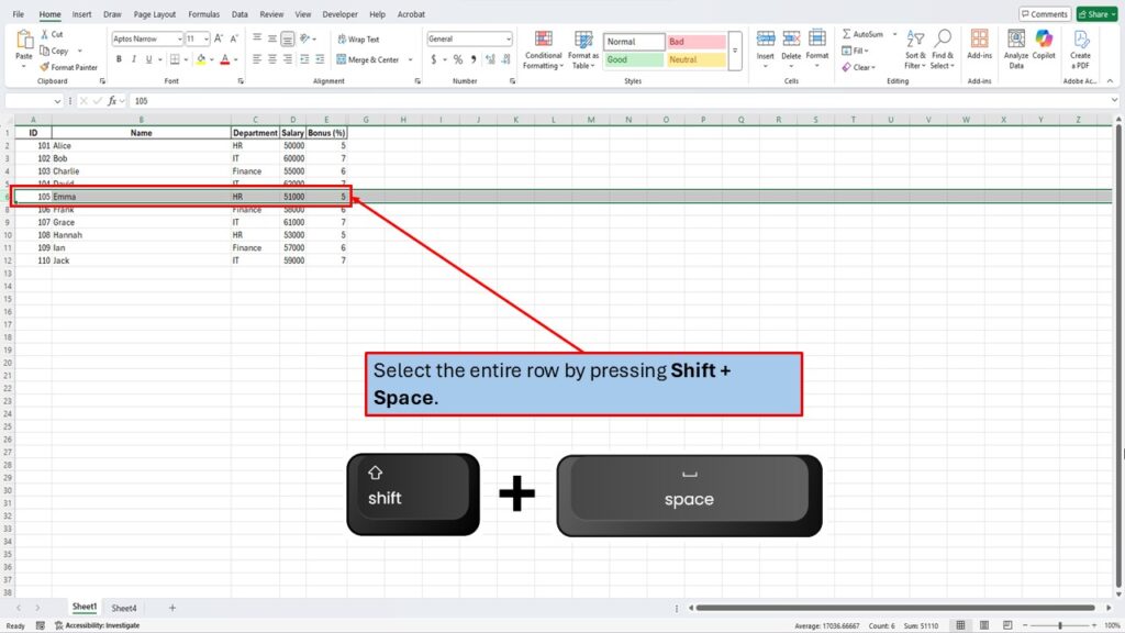
2. Select the Entire Row:
Once you’ve positioned the cursor in the desired row, press Shift + Space. This action selects the entire row, ensuring that any operations you perform will affect the whole row.
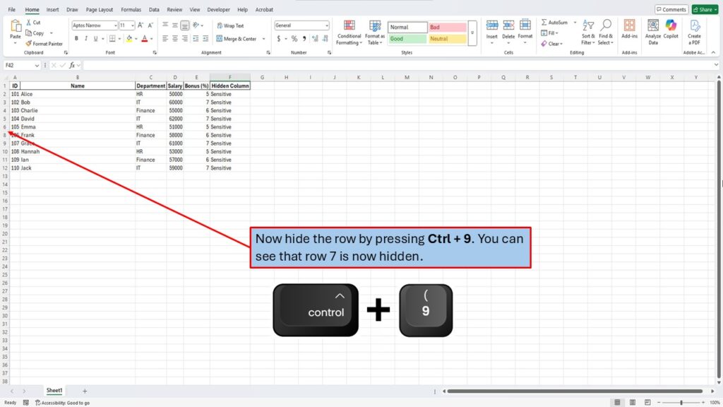
3. Hide the Selected Row:
With the row selected, press Ctrl + 9. This shortcut instantly hides the selected row from view.
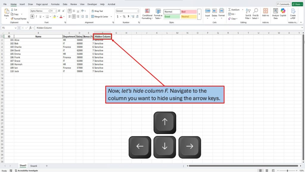
4. Navigate to the Column to Hide:
Decide which column you wish to hide, such as column F. Use the arrow keys to move to any cell within that column.
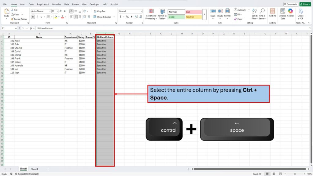
5. Select the Entire Column:
Press Ctrl + Space to select the entire column. This ensures that any subsequent actions will apply to the whole column.
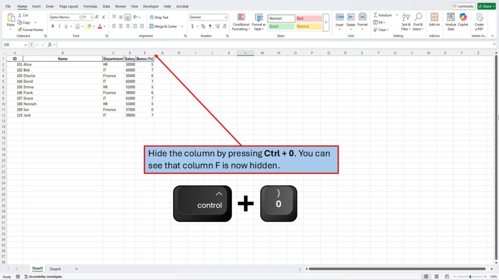
6. Hide the Selected Column:
With the column selected, press Ctrl + 0. This shortcut hides the selected column from your worksheet.
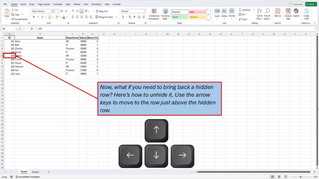
7. Prepare to Unhide a Hidden Row:
To unhide a row, first navigate to the row immediately above the hidden one using the arrow keys. For example, if row 7 is hidden, move to any cell in row 6.
8. Select the Adjacent Row Above:
Press Shift + Space to select the entire row above the hidden one.
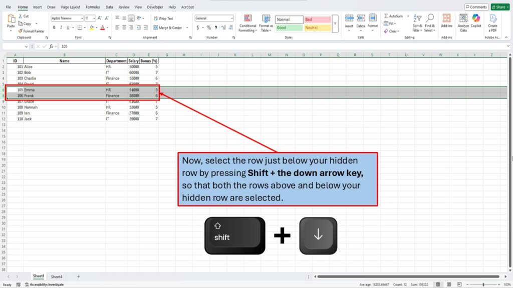
9. Extend Selection to the Row Below:
Hold down the Shift key and press the down arrow key to include the row below the hidden one in your selection. This means both the rows immediately above and below the hidden row are now selected.
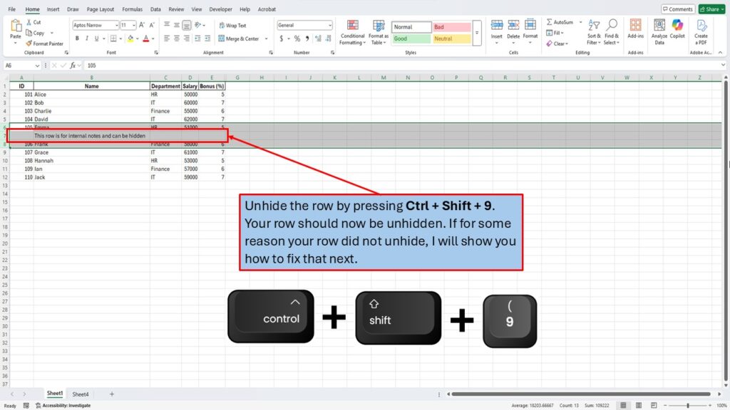
10. Unhide the Hidden Row:
Press Ctrl + Shift + 9. This command unhides any hidden rows within the selected range.
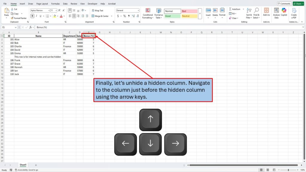
11. Navigate to the Columns Adjacent to the Hidden Column:
To unhide a hidden column, move to the column immediately before it. For instance, if column F is hidden, navigate to any cell in column E.
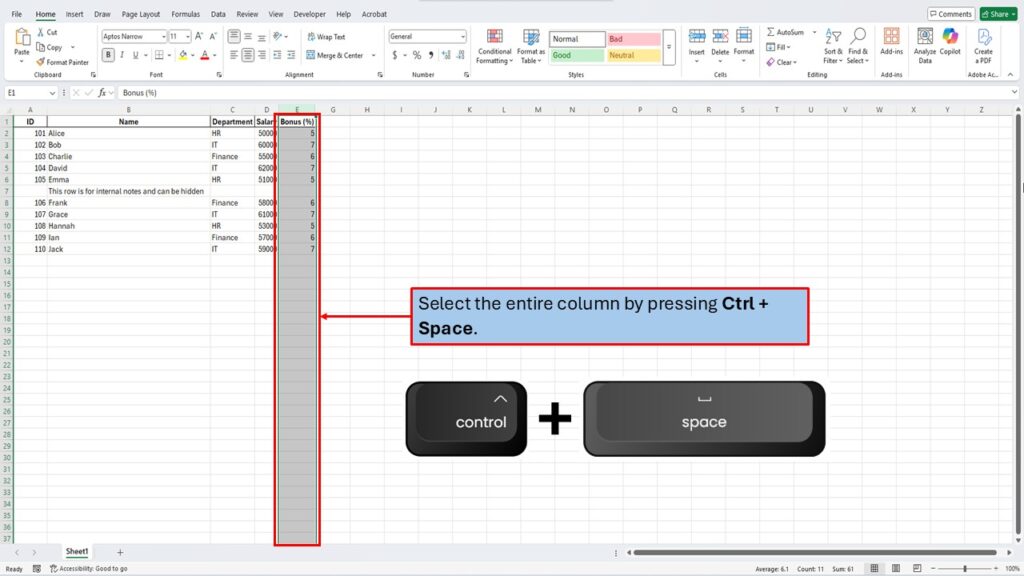
12. Select the Adjacent Column Before the Hidden One:
Press Ctrl + Space to select the entire column before the hidden one.
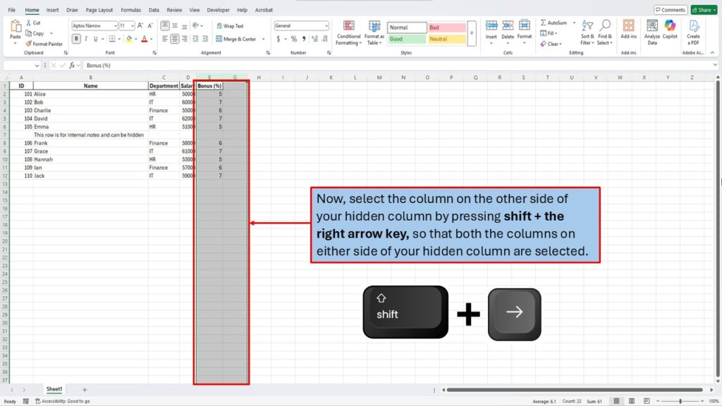
13. Extend Selection to the Column After the Hidden One:
Hold down the Shift key and press the right arrow key to include the column immediately after the hidden one in your selection. Now, both columns adjacent to the hidden column are selected.
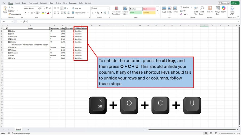
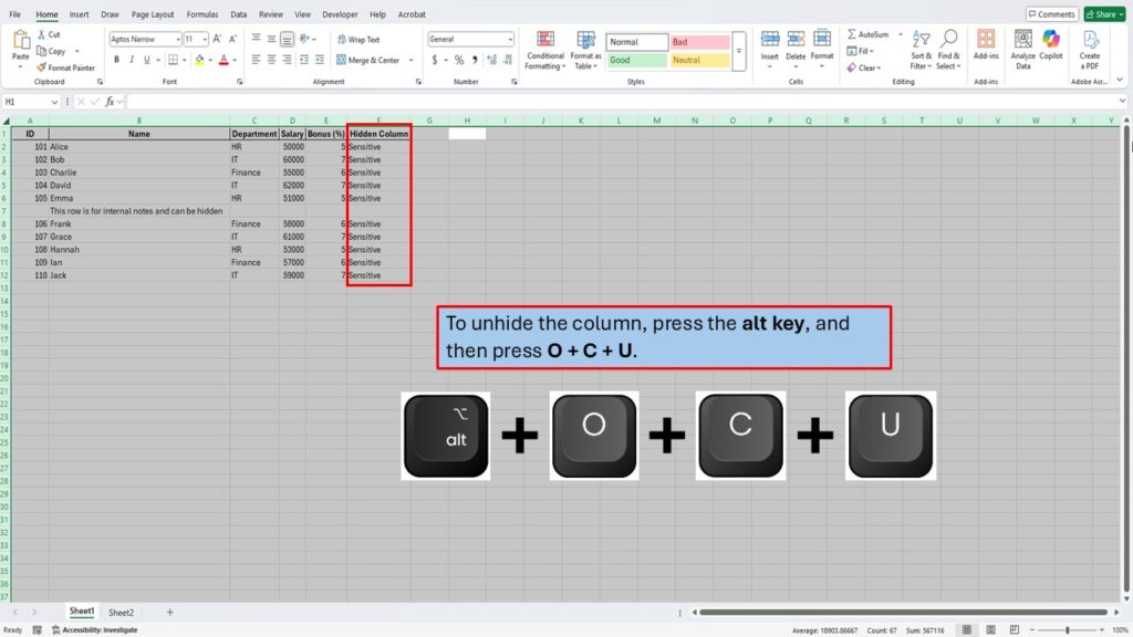
14. Unhide the Hidden Column:
Press the Alt key, then sequentially press H +O + U + L. This series of keystrokes accesses the ‘Home’ tab, opens the ‘Format’ menu, selects ‘Hide & Unhide’, and finally chooses ‘Unhide Columns’.
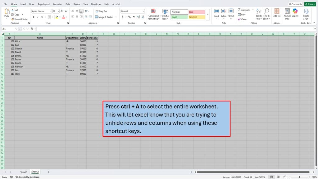
15. Select the Entire Worksheet if Unhiding Fails:
If the previous steps don’t unhide the rows or columns, press Ctrl + A to select the entire worksheet. This action ensures that Excel recognizes you’re attempting to unhide all hidden rows and columns.
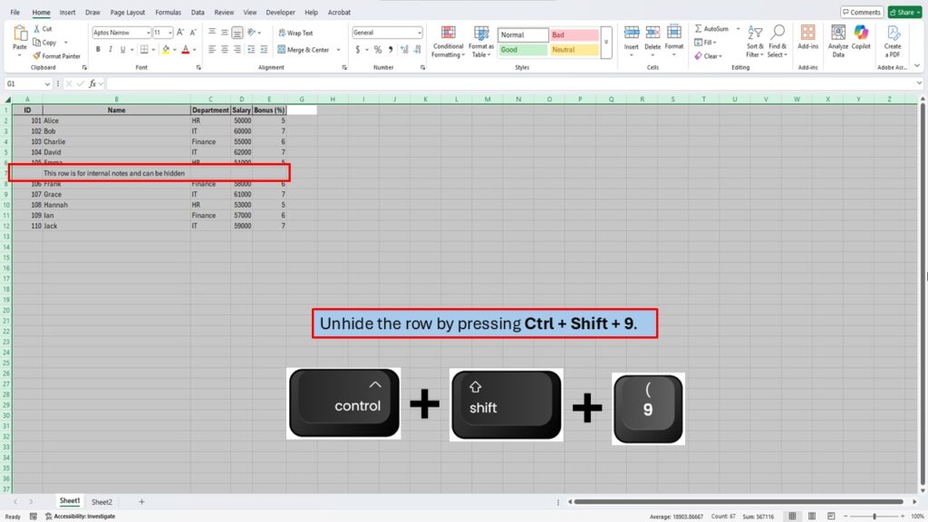
16. Unhide All Hidden Rows:
With the entire worksheet selected, press Ctrl + Shift + 9 to unhide all hidden rows.
17. Unhide All Hidden Columns:
Finally, to unhide all hidden columns, press the Alt key, then sequentially press H +O + U + L. This ensures that any hidden columns in the worksheet become visible again.
Need More Help?
Video Tutorial
Download PDF Below
View Our Latest Post Here: Master Excel Navigation: Alt Key Shortcuts Made Simple!