
Click here to view our video tutorial.
Click here to download our PDF tutorial.
Hello, and welcome to Mark’s Excel Tips. Today, we are going to show you two ways to wrap text in Excel. Let’s get started.
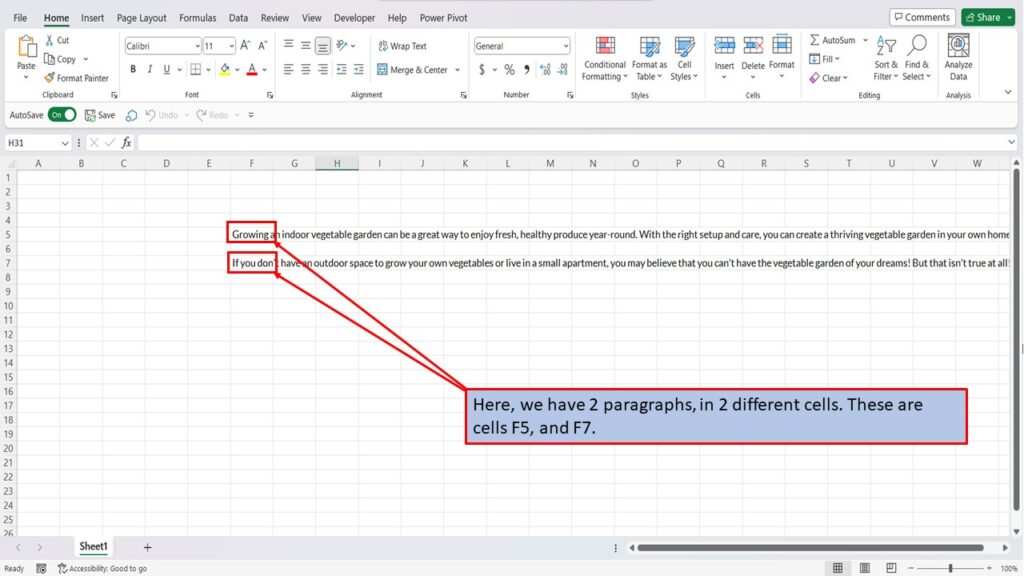
Here we have 2 paragraphs, in 2 different cells. These are cells F5, and F7.
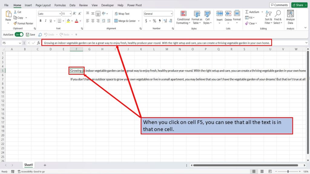
When you click on cell F5, you can see that all the text is in that one cell.
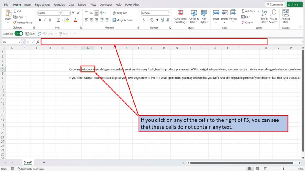
If you click on any of the cells to the right of F5, you can see that these cells do not contain any text.
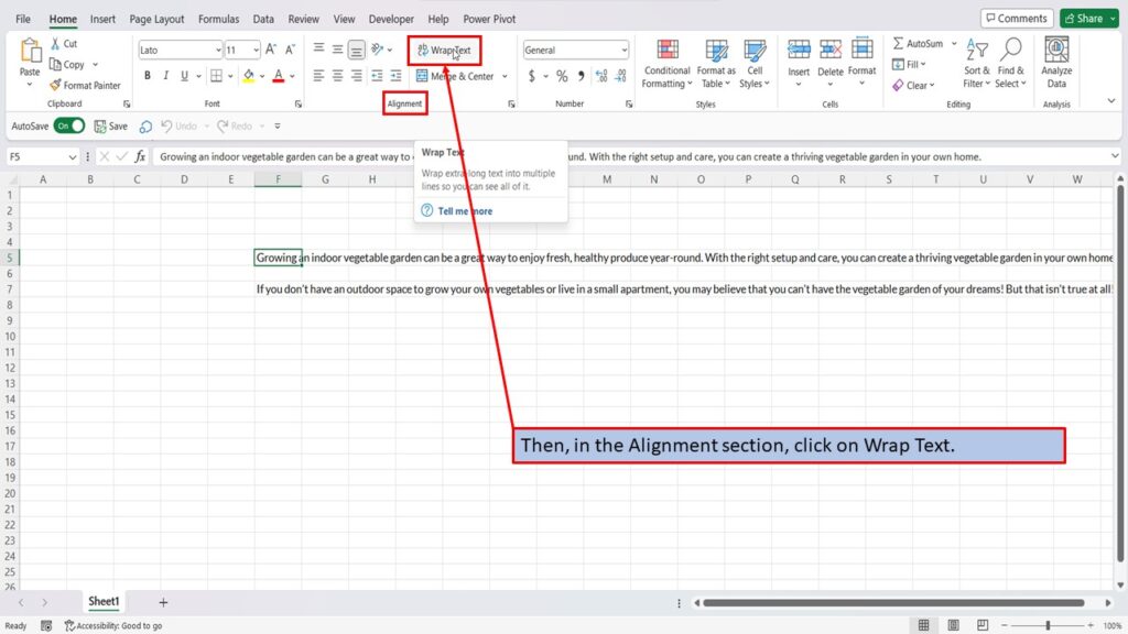
To wrap the text in cell F5. Click on that cell.
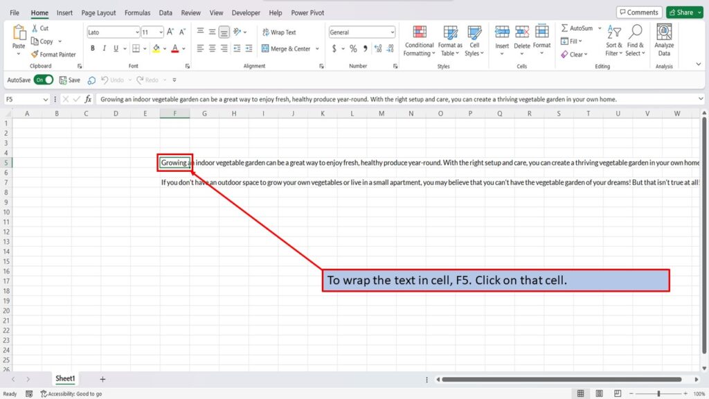
Then, in the Alignment section, click on Wrap Text.
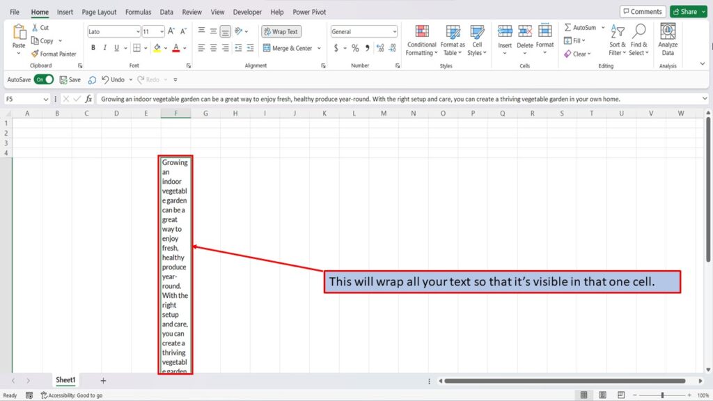
This will wrap all your text, so that it’s visible in that one cell.
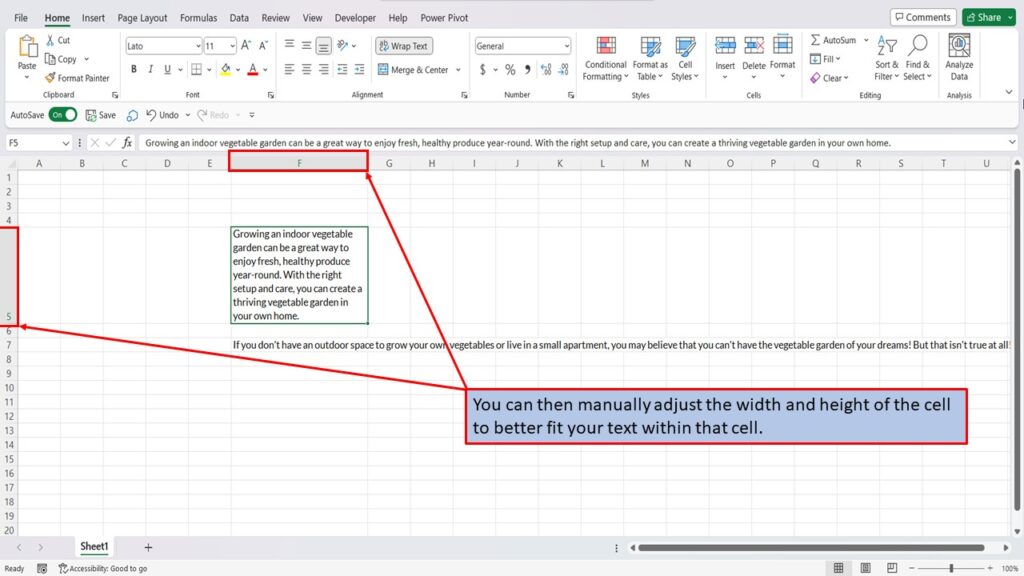
You can then manually adjust the width and height of the cell to better fit your text within that cell.
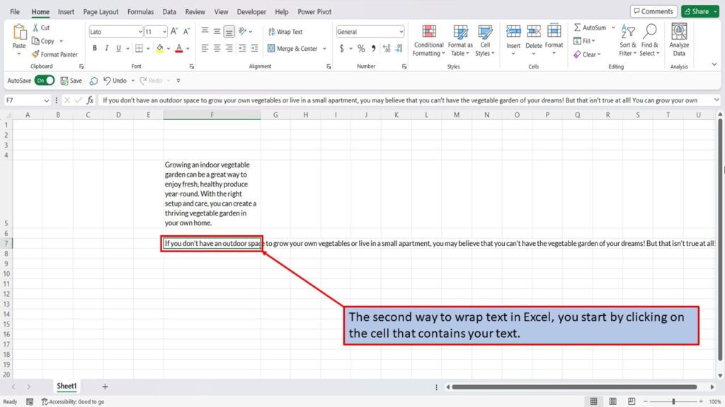
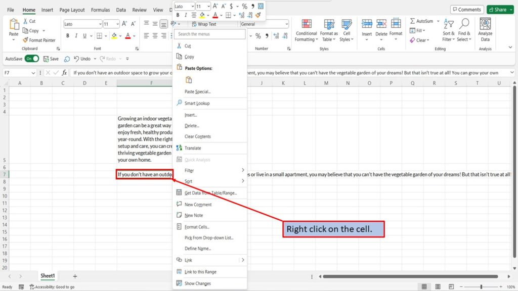
The second way to wrap text in Excel, is to start by clicking on the cell that contains your text.
Right click on the cell.
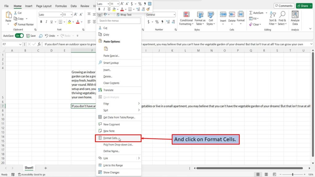
And click on Format Cells.
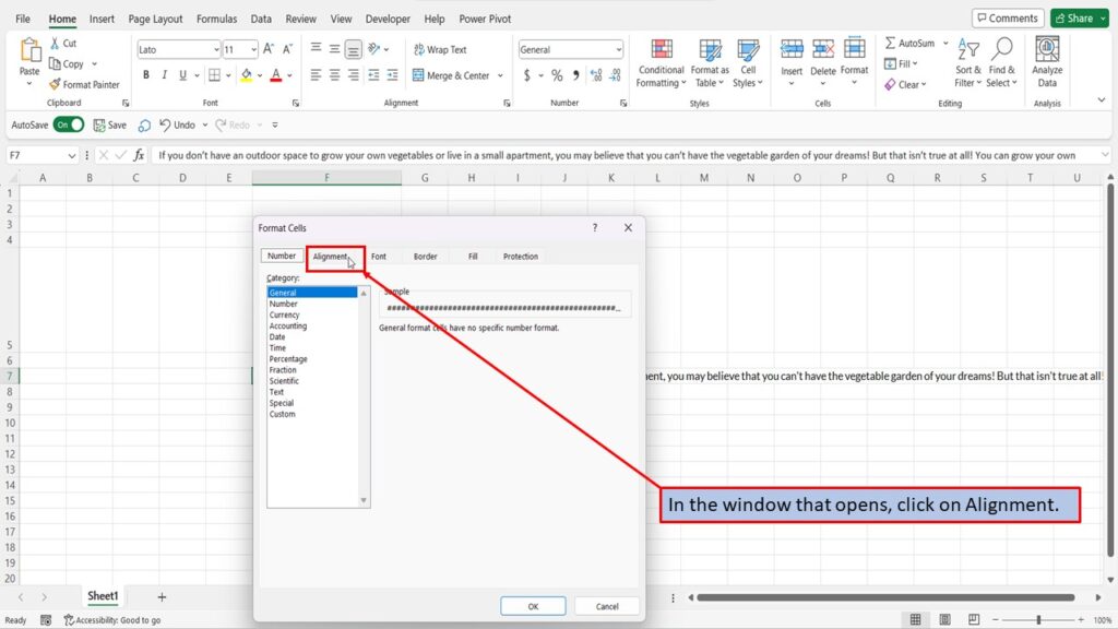
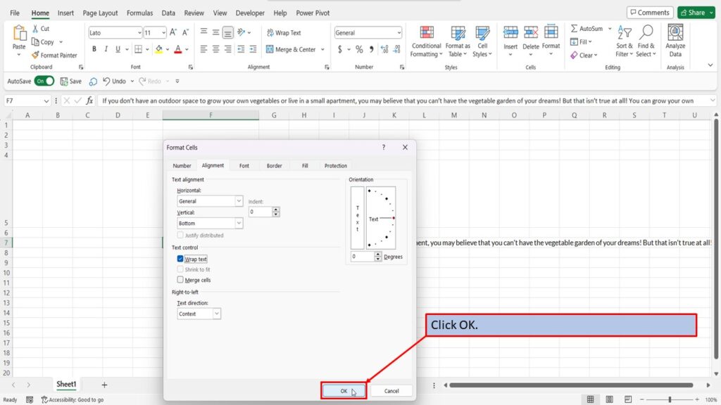
In the window that opens, click on Alignment.
Under Text control, check the box that says wrap text.
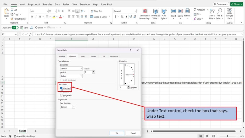
Click OK.
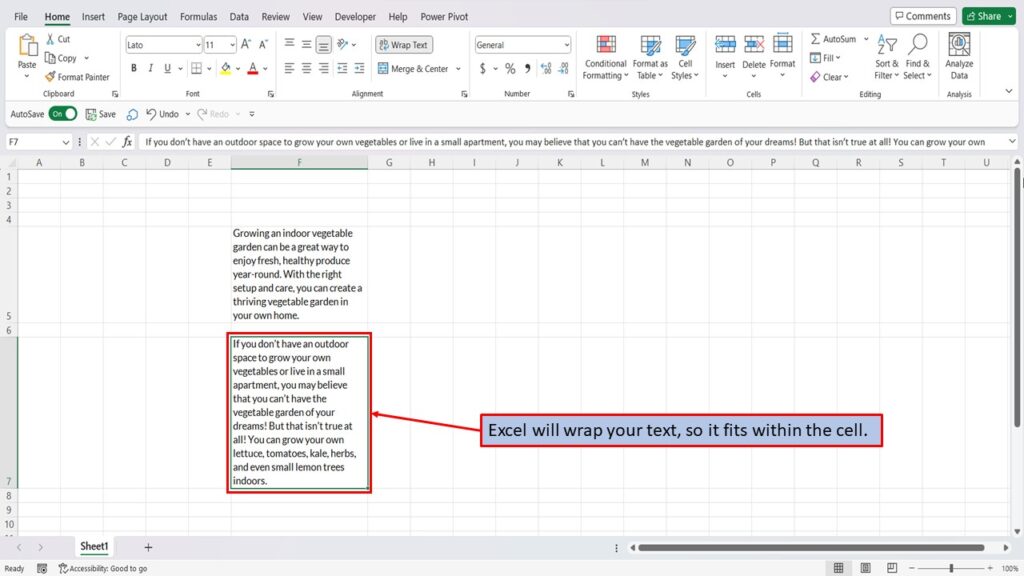
Excel will wrap your text, so it fits within the cell.
View the Video Tutorial.
Download this tutorial in PDF by clicking the Download link below.