
Hello, and welcome to Mark’s Excel Tips. Today, we are going to show you two ways, on how you can transpose data in Excel. Let’s get started.
Click here to view our video tutorial.
Click here to download our PDF tutorial.
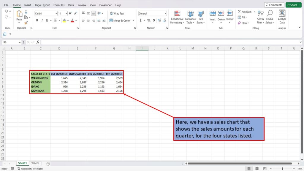
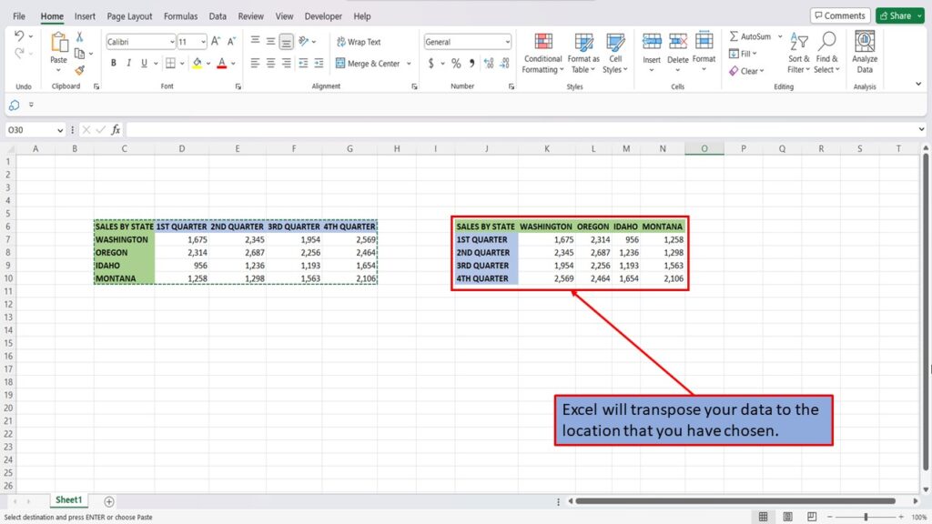
Here, we have a sales chart that shows the sales amounts for each quarter, for the four states listed.
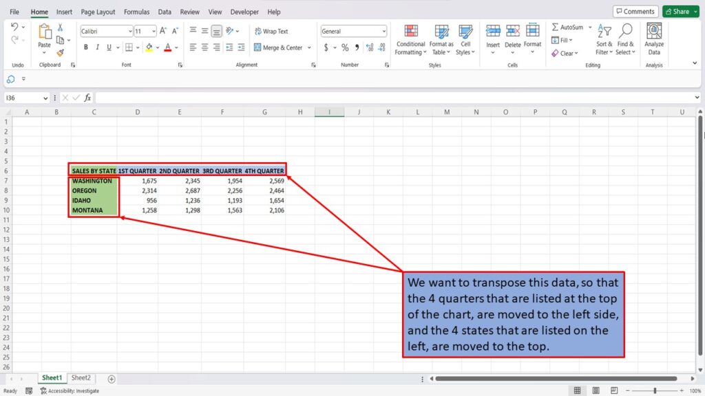
We want to transpose this data, so that the 4 quarters that are listed at the top of the chart, are moved to the left side, and the 4 states that are listed on the left, are moved to the top.
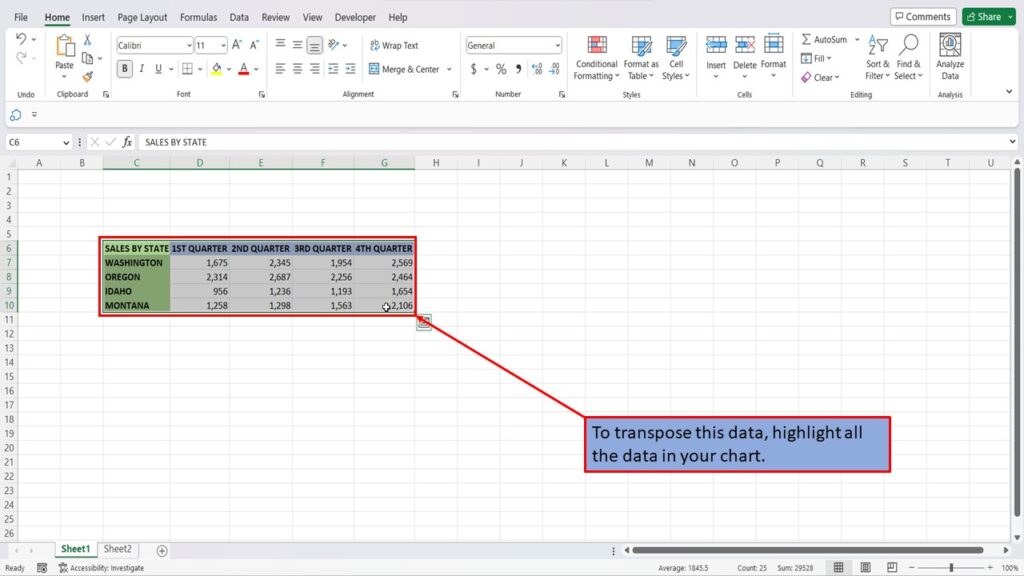
To transpose this data, highlight all the data in your chart.
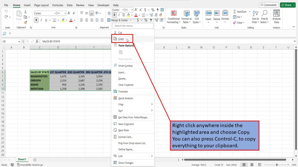
Right click anywhere inside the highlighted area and choose Copy. You can also press Control-C, to copy everything to your clipboard.
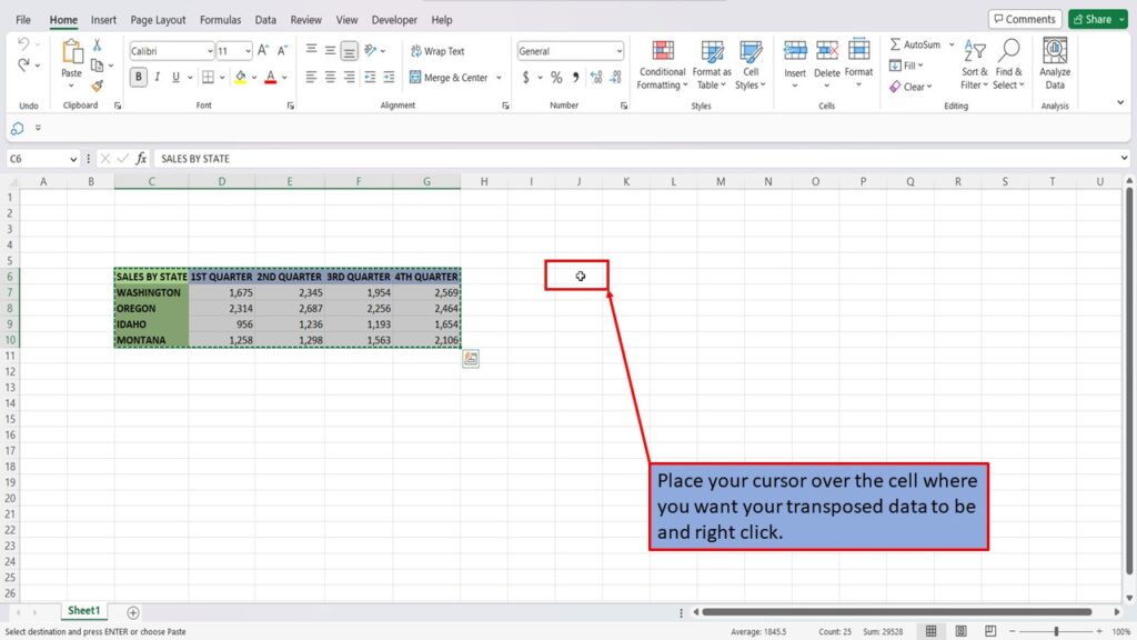
Place your cursor over the cell where you want your transposed data to be and right click.
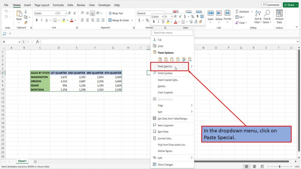
In the dropdown menu, click on Paste Special.
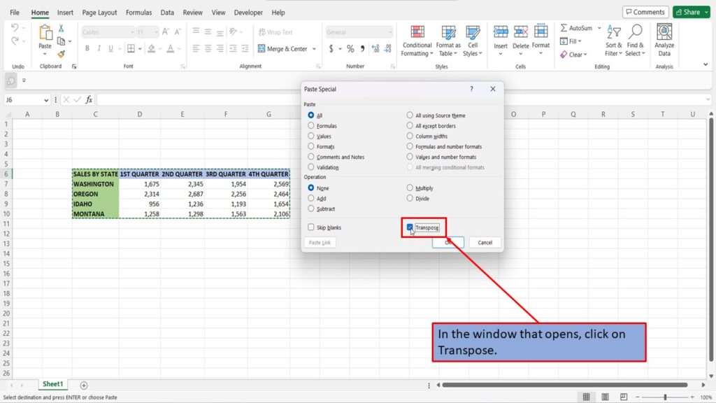
In the window that opens, click on Transpose.
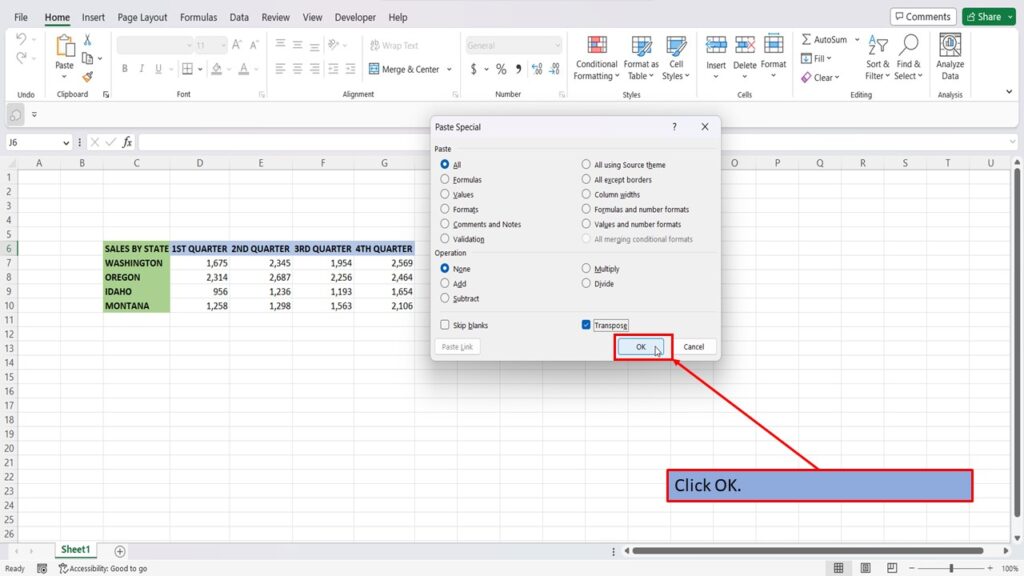
Click OK.
Excel will transpose your data to the location that you have chosen.
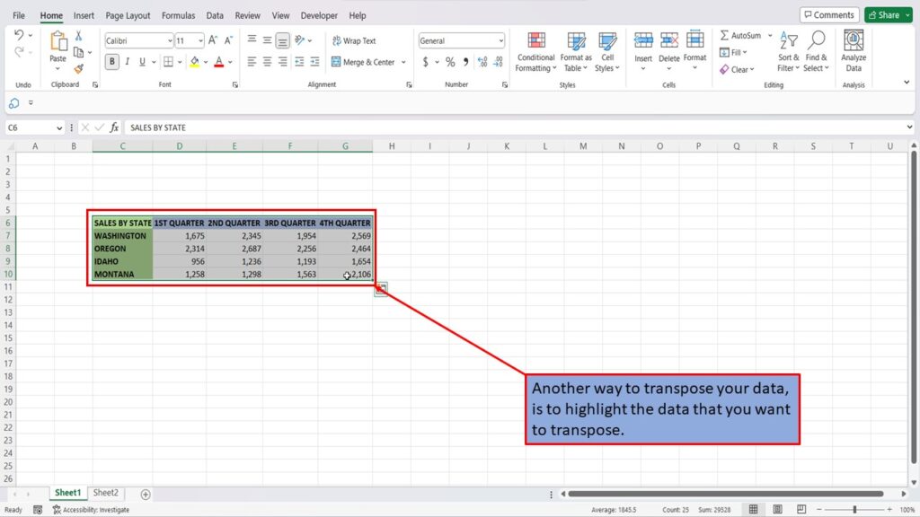
Another way to transpose your data, is to highlight the data that you want to transpose.
As before, right click anywhere inside the highlighted area and choose Copy. You can also press Control-C, to copy everything to your clipboard.

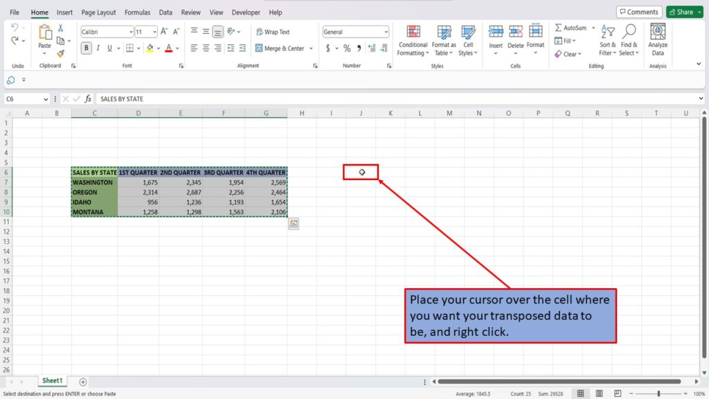
Place your cursor over the cell where you want your transposed data to be, and right click.
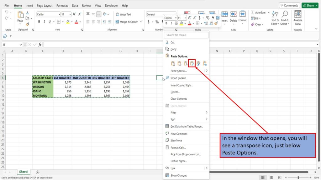
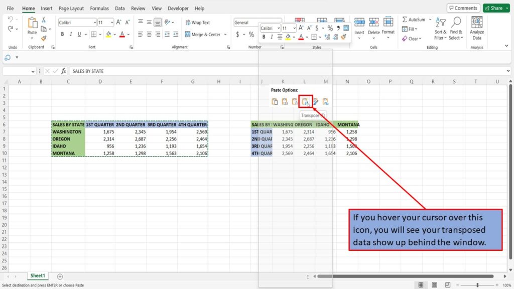
In the window that opens, you will see a transpose icon, just below Paste Options.
If you hover your cursor over this icon, you will see your transposed data show up behind the window.
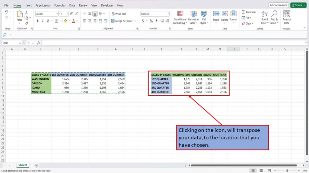
Clicking on the icon, will transpose your data, to the location that you have chosen.
View the Video Tutorial.
Download this tutorial in PDF by clicking the Download link below.