Click here to view our video tutorial.
Click here to download our PDF tutorial.
Hello, and welcome to Mark’s Excel Tips. Today, I will show you how to apply color, to alternate columns using conditional formatting in Excel 365. Let’s get started.
You first need to decide if you want to add color to alternating columns to the entire worksheet or just a specific area. If you want to add it to the entire worksheet, then click in the top left corner.

If you want to add color to just a specific area, then highlight that area.

Next, click on Home.

Click on Conditional Formatting.

In the dropdown menu, Click on New Rule.

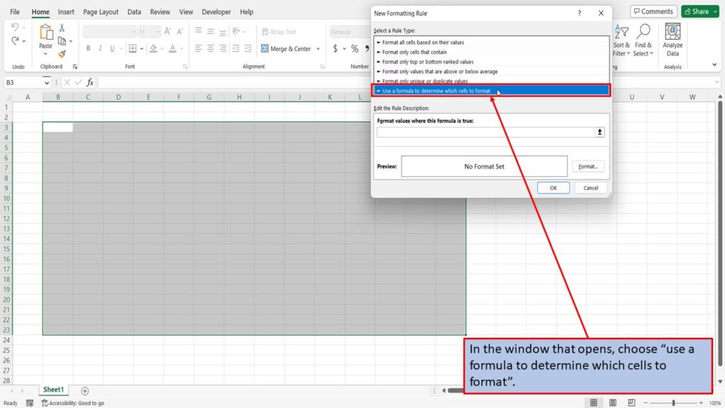
In the window that opens, choose “use a formula to determine which cells to format”.
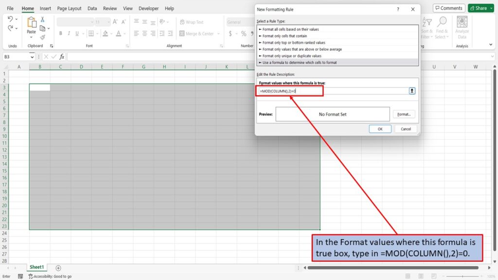
In the Format values where this formula is true box, type in =MOD(COLUMN(),2)=0.
Note: You can just copy and paste this formula into your worksheet.
Click on Format.

Next, click on Fill.

Click on the color that you want to use.

Click OK.

Click OK again.

Excel has applied alternating colors to your chosen columns.

View the vidio for this tutorial.
Download the PDF version of this tutorial by clicking download below.
